Page 508 - Fundamentals of Radar Signal Processing

Similarly combining these two equations gives the value of SNR, denoted by ,

required to achieve the specified probabilities when the interference estimate is
perfect:

(6.145)

The CFAR loss is then simply the ratio (Levanon, 1988; Hansen and Sawyers,
1980)

(6.146)

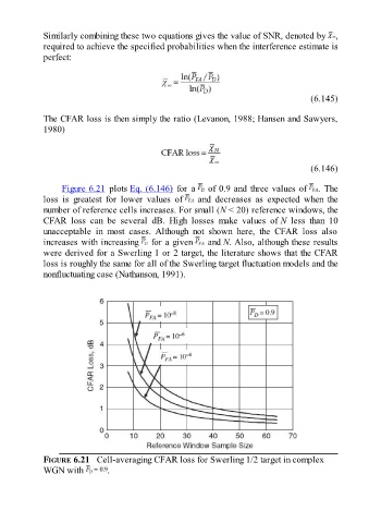
Figure 6.21 plots Eq. (6.146) for a of 0.9 and three values of . The
loss is greatest for lower values of and decreases as expected when the

number of reference cells increases. For small (N < 20) reference windows, the
CFAR loss can be several dB. High losses make values of N less than 10
unacceptable in most cases. Although not shown here, the CFAR loss also
increases with increasing for a given and N. Also, although these results
were derived for a Swerling 1 or 2 target, the literature shows that the CFAR
loss is roughly the same for all of the Swerling target fluctuation models and the
nonfluctuating case (Nathanson, 1991).

FIGURE 6.21 Cell-averaging CFAR loss for Swerling 1/2 target in complex
WGN with .