Page 231 - Fundamentals of Reservoir Engineering

OILWELL TESTING 169

q 3
q 1
q n
Rate q 2
q 4

time
t 1 t 2 t 3 t 4 t n

p i

p wf

time
t 1 t 2 t 3 t 4 t n
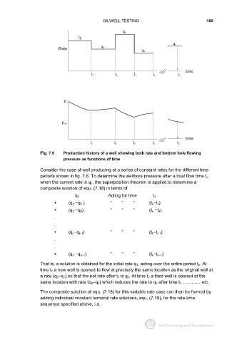
Fig. 7.6 Production history of a well showing both rate and bottom hole flowing
pressure as functions of time

Consider the case of well producing at a series of constant rates for the different time
periods shown in fig. 7.6. To determine the wellbore pressure after a total flow time t n
when the current rate is q n, the superposition theorem is applied to determine a
composite solution of equ. (7.18) in terms of

q 1 Acting for time t n
+ (q 2 −q 1 ) ” ” ” (t n−t 1)
+ (q 3 −q 2) ” ” ” (t n −t 2)
.
.

+ (q j −q j−1) ” ” ” (t n−t j−1)
.
.
+ (q n −q n−1) ” ” ” (t n−t n−1)

That is, a solution is obtained for the initial rate q 1, acting over the entire period t n. At
time t 1 a new well is opened to flow at precisely the same location as the original well at
a rate (q 2−q 1) so that the net rate after t 1 is q 2. At time t 2 a third well is opened at the
same location with rate (q 3−q 2) which reduces the rate to q 3 after time t 2 ………… etc.

The composite solution of equ. (7.18) for this variable rate case can then be formed by
adding individual constant terminal rate solutions, equ. (7.19), for the rate-time
sequence specified above, i.e.