Page 237 - Fundamentals of Reservoir Engineering

OILWELL TESTING 175

linear trend of the observed points on the Horner buildup plot will automatically match
equ. (7.37) as illustrated in fig. 7.9. Extrapolation of this line is useful in the
determination of the average reservoir pressure, Alternatively, an attempt can be made
to theoretically evaluate the p D function in the equation and then compare the
theoretical with the actual straight line with the aim of gaining additional information
about the reservoir. The application of this method will be illustrated in exercise 7.7.

If the well could be closed in for an infinite period of time the initial linear buildup would
typically follow the curved solid line in fig. 7.9 and could theoretically be predicted using
equ. (7.32). The final buildup pressure p is the average pressure within the bounded

volume being drained and is consistent with the material balance for this volume, i.e.

cAhφ (p − p) = qt (7.12)
i
which may be expressed as

2kh 2 khqt
π
π
( p − ) p = = 2π t DA (7.38)
i
µ
qµ q cA hφ
p*
equ. (7.37)
p ws

p
B
equ. (7.32)

A

small ∆t large ∆t
4 3 2 1 0
t + ∆t
In
∆t

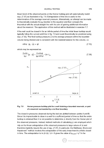
Fig. 7.9 Horner pressure buildup plot for a well draining a bounded reservoir, or part
of a reservoir surrounded by a no-flow boundary

The closed in pressures observed during the test are plotted between points A and B.
Since it is impracticable to close in a well for a sufficient period of time so that the entire
buildup is obtained then it is not possible to determine p directly from the Horner plot of
the observed pressures. Instead, indirect methods of calculating p are employed which
rely on the linear extrapolation of the observed pressures to large values of ∆t and
therefore implicitly require the use of equ. (7.37). In particular, the Matthews, Brons and
7
Hazebroek method involves the extrapolation of the early linear trend to infinite closed
*
in time. The extrapolation to In (t+∆t) / ∆t = 0 gives the value of p ws(LIN) = p In the