Page 238 - Fundamentals of Reservoir Engineering

OILWELL TESTING 176

particular case of a brief initial well test in a new reservoir the amount of fluids
withdrawn during the production phase will be infinitesimal and the extrapolated
*
pressure p will be equal to the initial pressure p i which is also the average pressure p.
This corresponds to the so-called infinite reservoir case for which p D (t D) in equ. (7.37)
may be evaluated under transient conditions, equ. (7.23), and hence the last two terms
*
in the former equation will cancel each other out. Apart from this special case p cannot
be thought of as having any clearly defined physical meaning but is merely a
mathematical device used in calculating the average reservoir pressure. Thus
evaluating equ. (7.37) for infinite closed in time gives
2kh ( p − p * ) = p (t ) − 1 ln 4t D (7.39)
π
qµ i D D 2 γ

and subtracting this equation from the material balance for the bounded drainage
volume, equ. (7.38), and multiplying throughout by 2, gives

4kh ( p − p = 4 π t + ln 4t D − 2p () (7.40)
π
*
)
t
qµ DA γ D D
*
Since p is obtained from the extrapolation of the observed pressure trend on the
Horner buildup plot, then p can be calculated once the right hand side of equ. (7.40)
has been correctly evaluated. This, of course, gets back to the old problem of how can
p D (t D), the dimensionless pressure, be determined for any value of t D, which is the
dimensionless flowing time prior to the survey? Matthews, Brons and Hazebroek
derived p D (t D) functions for a variety of bounded geometrical shapes and for wells
asymmetrically situated with respect to the boundary using the so-called "method of
images" with which the reader who has studied electrical potential field theory will
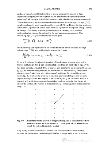
already be familiar. The method is illustrated for a 2 : 1 rectangular bounded reservoir
in fig. 7.10.

a
j

Fig. 7.10 Part of the infinite network of image wells required to simulate the no-flow
condition across the boundary of a 2 : 1 rectangular part of a reservoir in
which the real well is centrally located

Very briefly, in order to maintain a strict no-flow condition at the outer boundary
requires the placement of an infinite grid of virtual or image wells, a part of such an