Page 352 - Fundamentals of Reservoir Engineering

REAL GAS FLOW: GAS WELL TESTING 287

p
D(MBH)
m
D(MBH)
m
or D(MBH)
p
D(MBH)

(t ) SSS
DA

01 0.1 1.0 10.0

.00264 kt
t = φµ cA
DA
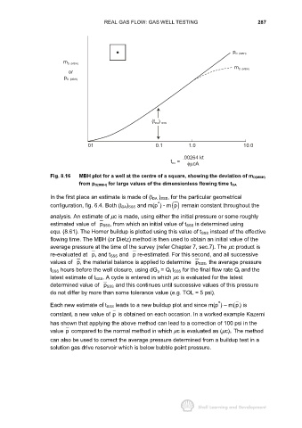
Fig. 8.16 MBH plot for a well at the centre of a square, showing the deviation of m D(MBH)

from p D(MBH) for large values of the dimensionless flowing time t DA

In the first place an estimate is made of (t DA ) SSS, for the particular geometrical
*
configuration, fig. 6.4. Both (t DA) SSS and m(p ) - m() p remain constant throughout the
analysis. An estimate of µc is made, using either the initial pressure or some roughly
estimated value of p SSS, from which an initial value of t SSS is determined using
equ. (8.61). The Horner buildup is plotted using this value of t SSS instead of the effective
flowing time. The MBH (or Dietz) method is then used to obtain an initial value of the
average pressure at the time of the survey (refer Chapter 7, sec.7). The µc product is
re-evaluated at p, and t SSS and p re-estimated. For this second, and all successive
values of p, the material balance is applied to determine p SSS, the average pressure
t SSS hours before the well closure, using dG p = Q l t SSS for the final flow rate Q l and the
latest estimate of t SSS. A cycle is entered in which µc is evaluated for the latest
determined value of p SSS and this continues until successive values of this pressure
do not differ by more than some tolerance value (e.g. TOL = 5 psi).

*
Each new estimate of t SSS leads to a new buildup plot and since m(p ) – m(p) is
constant, a new value of p is obtained on each occasion. In a worked example Kazemi

has shown that applying the above method can lead to a correction of 100 psi in the
value p compared to the normal method in which µc is evaluated as (µc) i. The method
can also be used to correct the average pressure determined from a buildup test in a
solution gas drive reservoir which is below bubble point pressure.