Page 174 - Fundamentals of The Finite Element Method for Heat and Fluid Flow

TRANSIENT HEAT CONDUCTION ANALYSIS
166
where c f is the specific heat in the freezing interval, L is the latent heat and T r is a
reference temperature that is below T s .
One of the earliest and most commonly used methods for solving such problems has
been the ‘effective heat capacity’ method. This method is derived from writing
2
∂H ∂H ∂T ∂ T
= = k in
(6.63)
∂t ∂T ∂t ∂x 2
We can rewrite the above equation as
2
∂T ∂ T
c eff = k 2 (6.64)
∂t ∂x
where c eff = ∂H/∂T is the effective heat capacity. This can be evaluated directly from
Equation 6.62 as
c eff = ρc s (T < T s )
L
c eff = ρc f + (T s <T <T l )
T l − T s
c eff = ρc l (T > T l ) (6.65)
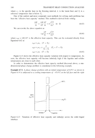
Figure 6.13 shows the effective heat capacity variation with respect to temperature. As
seen, the effective heat capacity will become infinitely high if the liquidus and solidus
temperatures are close to each other.
In order to demonstrate the effective heat capacity method discussed above, a one-
dimensional phase change problem is considered in the following example.
Example 6.7.1 A phase change problem with an initial temperature of 0.0 C as shown in
◦
◦
Figure 6.14 is subjected to a cooling temperature of −45.0 C at the left face and the right

H(T)

H(T)
rc (T)
p
(T)
rc p

x
Solidus Liquidus

Figure 6.13 Variation of effective heat capacity and enthalpy across the solid–liquid
interface