Page 170 - Fundamentals of The Finite Element Method for Heat and Fluid Flow

TRANSIENT HEAT CONDUCTION ANALYSIS
162
step is given as
t ≤ l 2 (6.55)
bα
where l is the element size and α is the thermal diffusivity.
Central Difference: The central difference approximation of the time term, with an explicit
treatment for the other terms, is unconditionally unstable, and this scheme is not recom-
mended.
Crank–Nicolson Scheme (semi-implicit): Owing to the oscillatory behaviour of this semi-
implicit scheme at larger time steps, it is often termed as a marginally stable scheme.

6.6 Multi-dimensional Transient Heat Conduction

A finite element solution for multi-dimensional problems follows the same procedure as that
for a one-dimensional case. However, the matrices [C], [K]and {f} are different because
of their multi-dimensions. For more details on the matrices, the reader should refer to
Chapter 3. A numerical problem, using a two- and three-dimensional approximation, is
solved in the following example.

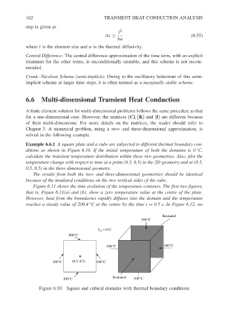
Example 6.6.1 A square plate and a cube are subjected to different thermal boundary con-
◦
ditions as shown in Figure 6.10. If the initial temperature of both the domains is 0 C,
calculate the transient temperature distribution within these two geometries. Also, plot the
temperature change with respect to time at a point (0.5, 0.5) in the 2D geometry and at (0.5,
0.5, 0.5) in the three-dimensional geometry.
The results from both the two- and three-dimensional geometries should be identical
because of the insulated conditions on the two vertical sides of the cube.
Figure 6.11 shows the time evolution of the temperature contours. The first two figures,
that is, Figure 6.11(a) and (b), show a zero temperature value at the centre of the plate.
However, heat from the boundaries rapidly diffuses into the domain and the temperature
reaches a steady value of 200.4 C at the centre by the time t = 0.5 s. In Figure 6.12, we
◦
Insulated
500°C

T o = 0°C
500°C

100°C 100°C

100°C (0.5, 0.5) 100°C

Insulated
100°C 100°C
Figure 6.10 Square and cubical domains with thermal boundary conditions