Page 166 - Fundamentals of The Finite Element Method for Heat and Fluid Flow

TRANSIENT HEAT CONDUCTION ANALYSIS
158
2 cm
T = 25°C
2
h = 200 W/m °C
1 2 3 Insulated
100°C
x

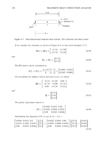
Figure 6.4 One-dimensional transient heat transfer. Two elements and three nodes

If we consider two elements, as shown in Figure 6.4, we have from Example 3.5.1,

0.124 −0.118
[K] 1 = [K] 2 = (6.39)
−0.118 0.124
and

0.15
{f} 1 ={f} 2 = (6.40)
0.15
The [C] matrix can be calculated as

ρc p AL 21 0.0484 0.0242
[C] 1 = [C] 2 = = (6.41)
6 12 0.0242 0.0484
On assembling the stiffness matrix and load vector, we obtain

 
0.124 −0.118 0.00
[K] =  −0.118 0.248 −0.118  (6.42)
0.00 −0.118 0.124

and  
0.15
{f}= 0.30 (6.43)
0.15
 
The global capacitance matrix is

0.0484 0.0242 0.00
 
[C] =  0.0242 0.0968 0.0242  (6.44)
0.00 0.0242 0.0484
Substituting into Equation 6.38, we get at t = 0.1 s

         
0.0546 0.0183 0.0 0.0422 0.0301 0.00
T 1 25.0 0.015
0.0183 0.1092 0.0183 0.0301 0.0844 0.0301 25.0 0.030
  T 2 =   +
0.00 0.0183 0.0546   0.00 0.0301 0.0422  25.0   0.015 
T 3
(6.45)