Page 164 - Fundamentals of The Finite Element Method for Heat and Fluid Flow

156
where P is the perimeter of the one-dimensional body. Substituting Equations 6.28 to 6.30
into Equation 6.16, for a domain with only one element, gives
∂T i
  TRANSIENT HEAT CONDUCTION ANALYSIS
 
ρc p lA 21  ∂t  Ak x 1 −1 hP l 21 T i
+ +
6 l −11 6 12 T j
12 ∂T j 
 
∂t

GAl 1 qP l 1 hT a Pl 1
= − + (6.31)
2 1 2 1 2 1
The above equation is a general representation of a one-dimensional problem with one
linear element. All the terms are included irrespective of whether or not boundary fluxes
and heat generation are present. We shall appropriately modify Equation 6.31, when solving
the numerical problems.
Equation 6.31 is semi-discrete as it is discretized only in space. We now require a
method of discretizing the transient terms of Equation 6.31. The following subsections
give the details of how the transient terms will be discretized.
6.4.1 Time discretization using the Finite Difference Method (FDM)

As may be seen from the semi-discrete form of Equation 6.31 (or 6.16), the differential
operator involving the time-dependent term still remains to be discretized. In this section, a
numerical approximation of the transient terms, using the Finite Difference Method (FDM),
is considered.
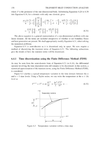
Figure 6.3 clarifies a typical temperature variation in the time domain between the n
and n + 1 time levels. Using a Taylor series, we can write the temperature at the n + 1th
level as
2
2
∂T n t ∂ T n
n
T n+1 = T + t + + ··· (6.32)
∂t 2 ∂t 2
T
Temperature variation

T n + 1
∆T
T n

t
t n t n + 1
∆t

Figure 6.3 Temperature variation within a time step