Page 167 - Fundamentals of The Finite Element Method for Heat and Fluid Flow

TRANSIENT HEAT CONDUCTION ANALYSIS
◦
From the second and third equations of the above system, we calculate that T 2 = 11.69 C
◦
and T 3 = 29.45 C.
Similarly at time t = 0.2 s, we arrive at the following values: 159
         
0.0546 0.0183 0.0 0.0422 0.0301 0.00
T 1 100.0 0.015
0.0183 0.1092 0.0183 0.0301 0.0844 0.0301 11.69 0.030
  T 2 =   +
0.00 0.0183 0.0546   0.00 0.0301 0.0422  29.45   0.015 
T 3
(6.46)
◦
◦
Solution of the above system results in T 2 = 24.68 C and T 3 = 21.22 C. It is observed
that the solution exhibits spatial and temporal oscillation at the start of the calculations.
These oscillations can be eliminated via suitable mesh refinement.
In the above example, it has been demonstrated how the transient solution is calculated.
In the following example, a similar case is considered using an explicit computer program
(see Chapter 10).
◦
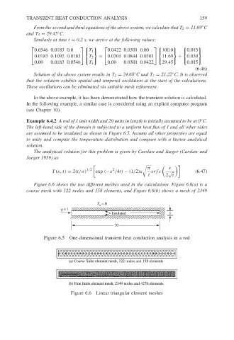
Example 6.4.2 A rod of 1 unit width and 20 units in length is initially assumed to be at 0 C.
The left-hand side of the domain is subjected to a uniform heat flux of 1 and all other sides
are assumed to be insulated as shown in Figure 6.5. Assume all other properties are equal
to unity and compute the temperature distribution and compare with a known analytical
solution.
The analytical solution for this problem is given by Carslaw and Jaeger (Carslaw and
Jaeger 1959) as

'
π x
2
T(x, t) = 2(t/π) 1/2 exp (−x /4t) − (1/2)x erf c √ (6.47)
t 2 t
Figure 6.6 shows the two different meshes used in the calculations. Figure 6.6(a) is a
coarse mesh with 122 nodes and 158 elements, and Figure 6.6(b) shows a mesh of 2349

T = 0
o
q = 1
Insulated 1

20

Figure 6.5 One-dimensional transient heat conduction analysis in a rod

(a) Coarse finite element mesh, 122 nodes and 158 elements

(b) Fine finite element mesh, 2349 nodes and 4276 elements

Figure 6.6 Linear triangular element meshes