Page 168 - Fundamentals of The Finite Element Method for Heat and Fluid Flow

TRANSIENT HEAT CONDUCTION ANALYSIS
160
(a) Temperature distribution on the coarse mesh, T max = 1.12 at the right-hand face
(b) Temperature distribution on the fine mesh, T max = 1.128 at the left-hand face

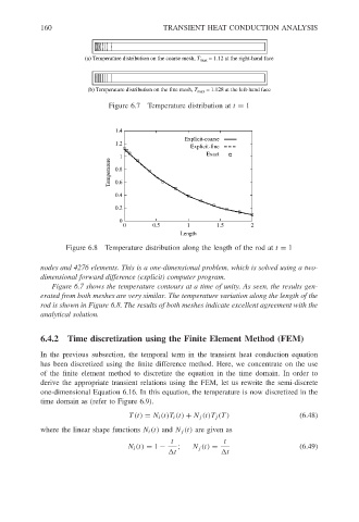
Figure 6.7 Temperature distribution at t = 1

1.4
Explicit-coarse
1.2
Explicit-fine
1 Exact
Temperature 0.8

0.6
0.4
0.2
0
0 0.5 1 1.5 2
Length
Figure 6.8 Temperature distribution along the length of the rod at t = 1

nodes and 4276 elements. This is a one-dimensional problem, which is solved using a two-
dimensional forward difference (explicit) computer program.
Figure 6.7 shows the temperature contours at a time of unity. As seen, the results gen-
erated from both meshes are very similar. The temperature variation along the length of the
rod is shown in Figure 6.8. The results of both meshes indicate excellent agreement with the
analytical solution.

6.4.2 Time discretization using the Finite Element Method (FEM)

In the previous subsection, the temporal term in the transient heat conduction equation
has been discretized using the finite difference method. Here, we concentrate on the use
of the finite element method to discretize the equation in the time domain. In order to
derive the appropriate transient relations using the FEM, let us rewrite the semi-discrete
one-dimensional Equation 6.16. In this equation, the temperature is now discretized in the
time domain as (refer to Figure 6.9).
T(t) = N i (t)T i (t) + N j (t)T j (T ) (6.48)

where the linear shape functions N i (t) and N j (t) are given as
t t
N i (t) = 1 − ; N j (t) = (6.49)
t t