Page 169 - Fundamentals of The Finite Element Method for Heat and Fluid Flow

TRANSIENT HEAT CONDUCTION ANALYSIS
T i (t)
i
N i (t) T j (t) j 161
N j (t)
∆t
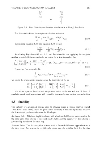
Figure 6.9 Time discretization between nth (i)and n + 1th (j) time levels

The time derivative of the temperature is thus written as
dT(t) dN i (t) dN j (t)
= T i (t) + T j (t) (6.50)
dt dt dt
Substituting Equation 6.49 into Equation 6.50, we get
dT(t) 1 1
=− T i (t) + T j (t) (6.51)
dt t t
Substituting Equations 6.48 and 6.51 into Equation 6.16 and applying the weighted
residual principle (Galerkin method), we obtain for a time interval of t,

N i (t) T i (t) T j (t) ( )
[C] − + + [K] N i (t)T i (t) + N j (t)T j (t) −{f} dt = 0
N j (t) t t
t
(6.52)
Employing (see Appendix B)

a b a!b!
N i (t) N j (t) dt = t (6.53)
t (a + b + 1)!
we obtain the characteristic equation over the time interval t as

[C] −11 T i (t) [K] 21 T i (t) 1 f 1
+ = (6.54)
2 t −11 T j (t) 3 12 T j (t) 2 f 2
The above equation involves the temperature values at the nth and n + 1th level. A
quadratic variation of temperature with respect to time may be derived in a similar fashion.

6.5 Stability

The stability of a numerical scheme may be obtained using a Fourier analysis (Hirsch
1988; Lewis et al. 1996). Here, we give a brief summary of the stability-related issues of
the time-stepping schemes discussed in this chapter.
Backward Euler: This is an implicit scheme with a backward difference approximation for
the time term. This scheme is unconditionally stable and the accuracy of the scheme is
governed by the size of the time step.

Forward Euler: This is an explicit scheme with a forward difference approximation to
the time term. The scheme is conditionally stable and the stability limit for the time