Page 163 - Fundamentals of The Finite Element Method for Heat and Fluid Flow

TRANSIENT HEAT CONDUCTION ANALYSIS
i Cross-sectional area, A j 155
l

x

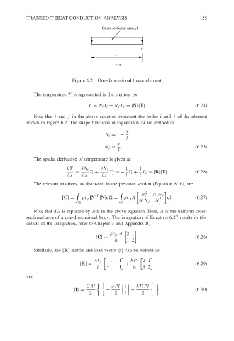
Figure 6.2 One-dimensional linear element

The temperature T is represented in the element by

T = N i T i + N j T j = [N]{T} (6.24)

Note that i and j in the above equation represent the nodes i and j of the element
shown in Figure 6.2. The shape functions in Equation 6.24 are defined as

x
N i = 1 −
l
x
N j = (6.25)
l
The spatial derivative of temperature is given as
∂T ∂N i ∂N j 1 1
= T i + T j =− T i + T j = [B]{T} (6.26)
∂x ∂x ∂x l l
The relevant matrices, as discussed in the previous section (Equation 6.16), are

2
T N i N i N j
[C] = ρc p [N] [N]d
= ρc p A 2 dl (6.27)

l N i N j N j
Note that d
is replaced by Adl in the above equation. Here, A is the uniform cross-
sectional area of a one-dimensional body. The integration of Equation 6.27 results in (for
details of the integration, refer to Chapter 3 and Appendix B)

ρc p lA 21
[C] = (6.28)
6 12
Similarly, the [K] matrix and load vector {f} can be written as

Ak x 1 −1 hP l 21
[K] = + (6.29)
l −1 1 6 12
and

GAl 1 qP l 1 hT a Pl 1
{f}= − + (6.30)
2 1 2 1 2 1