Page 239 - Fundamentals of The Finite Element Method for Heat and Fluid Flow

231
CONVECTION HEAT TRANSFER
Navier–Stokes equations on a mesh with element sizes very close to zero. The disadvantage of
DNS is that computing hardware is not yet available to tackle any reasonably sized practical
problem. The LES technique is computationally less intensive than DNS and results in a
time-dependent turbulent pattern, which is averaged in space. Currently available computing
resources can only just model small-scale 3D problems. The RANS method is the most widely
used turbulence modelling approach in the engineering industry due to the relatively small
number of nodes required to compute turbulence as compared to the DNS and LES techniques.
However,theresultsareaveragedoveratimescaleandthereforeonlytime-averagedquantities
are obtained from these models. The accuracy of the results are highly dependent on the model
and mesh employed. A detailed discussion on these methods is outside the scope of this book,
but interested readers should consult available text books and research papers on the topic
(Launder and Spalding 1972; Mohammadi and Pironneau 1994; Srinivas et al. 1994; Wilcox
1993; Wolfstein 1970; Zienkiewicz et al. 1996). However, a brief discussion on the RANS
approach is given below.
In the RANS approach, all variables in the Navier–Stokes equations are replaced by
the summation of an averaged value and the instantaneous variation, that is,
φ i = φ + φ i (7.194)
i

where φ is the instantaneous variation of φ and φ is a time-averaged value of φ given as
i
i
1 t
φ = φ i dt (7.195)
i
t 0
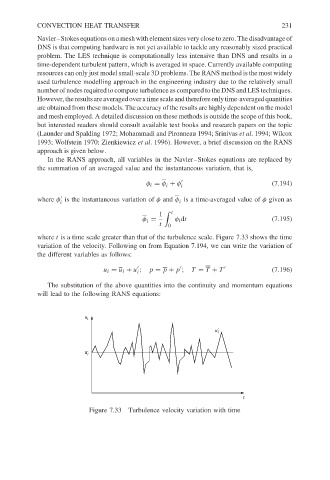
where t is a time scale greater than that of the turbulence scale. Figure 7.33 shows the time
variation of the velocity. Following on from Equation 7.194, we can write the variation of
the different variables as follows:

u i = u i + u ; p = p + p ; T = T + T (7.196)
i
The substitution of the above quantities into the continuity and momentum equations
will lead to the following RANS equations:

u i
u ’ i

u i

t
Figure 7.33 Turbulence velocity variation with time