Page 50 - Fundamentals of The Finite Element Method for Heat and Fluid Flow

42
x
i x j THE FINITE ELEMENT METHOD
i j k
l/2
l/2 x j
l x i x k
x i x j
(a) (b)

1 2 1 2
1 2 3 1 2 3 4 5
Linear Quadratic
approximation Approximation

Exact Exact

x x
− Element
− Node
(c) (d)
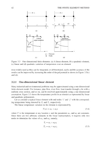
Figure 3.3 One-dimensional finite elements. (a) A linear element, (b) a quadratic element,
(c) linear and (d) quadratic variation of temperature over an element

most widely used as they can be integrated, or differentiated, easily and the accuracy of the
results can be improved by increasing the order of the polynomial as shown in Figure 3.3(c)
and (d).

3.2.1 One-dimensional linear element

Many industrial and environmental problems may be approximated using a one-dimensional
finite element model. For instance, pipe flow, river flow, heat transfer through a fin with a
uniform cross section, and so on, can be resolved approximately using a one-dimensional
assumption. Figure 3.3 shows the temperature profile in an element as represented by linear
and quadratic polynomials.
Let us consider a typical linear element with end nodes ‘i’ and ‘j’ with the correspond-
ing temperature being denoted by T i and T j respectively.
The linear temperature variation in the element is represented by

T(x) = α 1 + α 2 x (3.4)
where T is the temperature at any location x and the parameters α 1 ,and α 2 are constants.
Since there are two arbitrary constants in the linear representation, it requires only two
nodes to determine the values of α 1 ,and α 2 , namely,

T i = α 1 + α 2 x i

T j = α 1 + α 2 x j (3.5)