Page 52 - Fundamentals of The Finite Element Method for Heat and Fluid Flow

44
Shape function values
l N i N j l THE FINITE ELEMENT METHOD
within an element

i j
T j
Typical temperature
T i variation within an element
i j

dN /dx
j
Derivative of shape function
within an element
i dN i /dx j
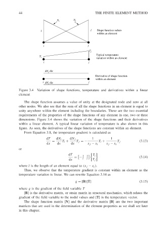
Figure 3.4 Variation of shape functions, temperature and derivatives within a linear
element

The shape function assumes a value of unity at the designated node and zero at all
other nodes. We also see that the sum of all the shape functions in an element is equal to
unity anywhere within the element including the boundaries. These are the two essential
requirements of the properties of the shape functions of any element in one, two or three
dimensions. Figure 3.4 shows the variation of the shape functions and their derivatives
within a linear element. A typical linear variation of temperature is also shown in this
figure. As seen, the derivatives of the shape functions are constant within an element.
From Equation 3.8, the temperature gradient is calculated as

dT dN i dN j 1 1
= T i + T j =− T i + T j (3.13)
dx dx dx x j − x i x j − x i
or
dT 1 1 T i

= − (3.14)
dx l l T j
where l is the length of an element equal to (x j − x i ).
Thus, we observe that the temperature gradient is constant within an element as the
temperature variation is linear. We can rewrite Equation 3.14 as

g = [B]{T} (3.15)
where g is the gradient of the field variable T
[B] is the derivative matrix, or strain matrix in structural mechanics, which relates the
gradient of the field variable to the nodal values and {T} is the temperature vector.
The shape function matrix [N] and the derivative matrix [B] are the two important
matrices that are used in the determination of the element properties as we shall see later
in this chapter.