Page 51 - Fundamentals of The Finite Element Method for Heat and Fluid Flow

THE FINITE ELEMENT METHOD
From the above equations, we get
T i x j − T j x i 43
α 1 =
x j − x i
T j − T i
α 2 = (3.6)
x j − x i
On substituting the values of α 1 ,and α 2 into Equation 3.4 we get

x j − x x − x i
T = T i + T j (3.7)
x j − x i x j − x i
or

T i

T = N i T i + N j T j = N i N j (3.8)
T j
where N i and N j are called Shape functions or Interpolation functions or Basis functions.

x j − x
N i =
x j − x i

x − x i
N j = (3.9)
x j − x i
Equation 3.8 can be rewritten as

T = [N]{T} (3.10)
where

[N] = N i N j (3.11)
is the shape function matrix and

T i
{T}= (3.12)
T j
is the vector of unknown temperatures.
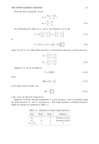
Equation 3.8 shows that the temperature T at any location x can be calculated using
the shape functions N i and N j evaluated at x. The shape functions at different locations
within an element are tabulated in Table 3.1.

Table 3.1 Properties of linear shape functions

Item Node, i Node, j Arbitrary x

N i 1 0 between 0 and 1
N j 0 1 between 0 and 1
N i + N j 1 1 1