Page 93 - Fundamentals of The Finite Element Method for Heat and Fluid Flow

85
THE FINITE ELEMENT METHOD
3.3.4 Galerkin finite element method
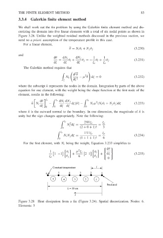
We shall work out the fin problem by using the Galerkin finite element method and dis-
cretizing the domain into five linear elements with a total of six nodal points as shown in
Figure 3.28. Unlike the weighted residual methods discussed in the previous section, we
need no a priori assumption of the temperature profile in this case.
For a linear element,
θ = N i θ i + N j θ j (3.230)
and
dθ dN i dN j 1 1
= θ i + θ j =− θ i + θ j (3.231)
dζ dζ dζ ζ e ζ e
The Galerkin method requires that
!
d θ 2
2
N k − µ θ dζ = 0 (3.232)
ζ dζ 2
where the subscript k represents the nodes in the domain. Integration by parts of the above
equation for one element, with the weight being the shape function at the first node of the
element, results in the following:
dθ dN i dN j 2
ζ e ζ e ζ e
˜ n N i − dζ{θ}− N i µ (N i θ i + N j θ j )dζ (3.233)
dζ dζ dζ
0 0 0
where ˜n is the outward normal to the boundary. In one dimension, the magnitude of ˜n is
unity but the sign changes appropriately. Note the following:
ζ e

2 2!0!ζ e ζ e
N dζ = =
i
0 (2 + 0 + 1)! 3
ζ e

1!1!ζ e ζ e
N i N j dζ = = (3.234)
0 (1 + 1 + 1)! 6
For the first element, with N i being the weight, Equation 3.233 simplifies to
dθ
 
2  
θ i µ ζ e θ i
1
1 −1 + 21 + dζ (3.235)
ζ e θ j 6 θ j  
0
Constant temperature l
6 5 4 3 2 1
5 4 3 2 1
Insulated
L = 10 cm
x
Figure 3.28 Heat dissipation from a fin (Figure 3.24). Spatial discretization. Nodes: 6.
Elements: 5