Page 95 - Fundamentals of The Finite Element Method for Heat and Fluid Flow

87
THE FINITE ELEMENT METHOD
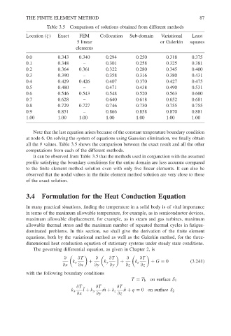
Table 3.5
Collocation
FEM
Variational
Sub-domain
Location (ζ) Exact Comparison of solutions obtained from different methods Least
5 linear or Galerkin squares
elements
0.0 0.343 0.340 0.294 0.250 0.318 0.375
0.1 0.348 – 0.301 0.258 0.325 0.381
0.2 0.364 0.361 0.322 0.280 0.345 0.400
0.3 0.390 – 0.358 0.316 0.380 0.431
0.4 0.429 0.426 0.407 0.370 0.427 0.475
0.5 0.480 – 0.471 0.438 0.490 0.531
0.6 0.546 0.543 0.548 0.520 0.563 0.600
0.7 0.628 – 0.640 0.618 0.652 0.681
0.8 0.729 0.727 0.746 0.730 0.755 0.755
0.9 0.851 – 0.866 0.858 0.870 0.881
1.00 1.00 1.00 1.00 1.00 1.00 1.00

Note that the last equation arises because of the constant temperature boundary condition
at node 6. On solving the system of equations using Gaussian elimination, we finally obtain
all the θ values. Table 3.5 shows the comparison between the exact result and all the other
computations from each of the different methods.
It can be observed from Table 3.5 that the methods used in conjunction with the assumed
profile satisfying the boundary conditions for the entire domain are less accurate compared
to the finite element method solution even with only five linear elements. It can also be
observed that the nodal values in the finite element method solution are very close to those
of the exact solution.

3.4 Formulation for the Heat Conduction Equation

In many practical situations, finding the temperature in a solid body is of vital importance
in terms of the maximum allowable temperature, for example, as in semiconductor devices,
maximum allowable displacement, for example, as in steam and gas turbines, maximum
allowable thermal stress and the maximum number of repeated thermal cycles in fatigue-
dominated problems. In this section, we shall give the derivation of the finite element
equations, both by the variational method as well as the Galerkin method, for the three-
dimensional heat conduction equation of stationary systems under steady state conditions.
The governing differential equation, as given in Chapter 2, is

∂ ∂T ∂ ∂T ∂ ∂T
k x + k y + k z + G = 0 (3.241)
∂x ∂x ∂y ∂y ∂z ∂z
with the following boundary conditions
T = T b on surface S 1
∂T ∂T ∂T
k x ˜ l + k y ˜ m + k z ˜ n + q = 0 on surface S 2
∂x ∂y ∂z