Page 622 - Fundamentals of Water Treatment Unit Processes : Physical, Chemical, and Biological

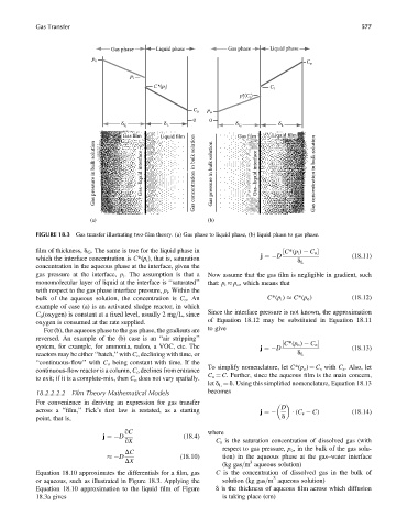
Gas Transfer 577

Gas phase Liquid phase Gas phase Liquid phase
p o C o

p i
C*(p ) C i
i
p*(C ) i
i
p
C o o
0 0
δ G δ L δ G δ L
Gas film Liquid film Gas film Liquid film
Gas pressure in bulk solution Gas–liquid interface Gas concentration in bulk solution Gas pressure in bulk solution Gas–liquid interface Gas concentration in bulk solution

(a) (b)
FIGURE 18.3 Gas transfer illustrating two-film theory. (a) Gas phase to liquid phase, (b) liquid phase to gas phase.

film of thickness, d G . The same is true for the liquid phase in ½ C*(p i ) C o Š
j ¼ D (18:11)
which the interface concentration is C*(p i ), that is, saturation
d L
concentration in the aqueous phase at the interface, given the
gas pressure at the interface, p i . The assumption is that a Now assume that the gas film is negligible in gradient, such
monomolecular layer of liquid at the interface is ‘‘saturated’’ that: p i p o , which means that
with respect to the gas phase interface pressure, p i . Within the
bulk of the aqueous solution, the concentration is C o .An C*(p i ) C*(p o ) (18:12)
example of case (a) is an activated sludge reactor, in which
Since the interface pressure is not known, the approximation
C o (oxygen) is constant at a fixed level, usually 2 mg=L, since
of Equation 18.12 may be substituted in Equation 18.11
oxygen is consumed at the rate supplied.
to give
For (b), the aqueous phase to the gas phase, the gradients are
reversed. An example of the (b) case is an ‘‘air stripping’’
system, for example, for ammonia, radon, a VOC, etc. The j ¼ D ½ C*(p o ) C o Š (18:13)
reactors may be either ‘‘batch,’’ with C o declining with time, or d L
‘‘continuous-flow’’ with C o being constant with time. If the
To simplify nomenclature, let C*(p o ) ¼ C s with C s . Also, let
continuous-flow reactor is a column, C o declines from entrance
C o ¼ C. Further, since the aqueous film is the main concern,
to exit; if it is a complete-mix, then C o does not vary spatially.
let d L ¼ d. Using this simplified nomenclature, Equation 18.13
18.2.2.2.2 Film Theory Mathematical Models becomes
For convenience in deriving an expression for gas transfer
D
across a ‘‘film,’’ Fick’s first law is restated, as a starting (C s C) (18:14)
j ¼
point, that is, d
qC where
j ¼ D (18:4)
qX C s is the saturation concentration of dissolved gas (with
respect to gas pressure, p o , in the bulk of the gas solu-
DC
D (18:10) tion) in the aqueous phase at the gas–water interface
DX 3
(kg gas=m aqueous solution)
Equation 18.10 approximates the differentials for a film, gas C is the concentration of dissolved gas in the bulk of
3
or aqueous, such as illustrated in Figure 18.3. Applying the solution (kg gas=m aqueous solution)
Equation 18.10 approximation to the liquid film of Figure d is the thickness of aqueous film across which diffusion
18.3a gives is taking place (cm)