Page 94 - Fundamentals of Water Treatment Unit Processes : Physical, Chemical, and Biological

Models 49

0.020

0.50
0.015
0.45
0.40
v(screen) (m/s) 0.010 0.25 0.30
0.35

0.15 0.20
0.005
0.10 rad/s

w= 0.05 rad/s
0.000
0.0 0.1 0.2 0.3 0.4 0.5
Headloss, h (m)

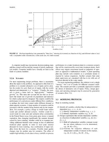
FIGURE 3.2 Plot from hypothetical data generated by ‘‘black box,’’ showing f [v(screen)] as a function of x(h L ) and different values of y(v)
with z (suspended solids concentration, screen mesh size, etc.) held constant.

A computer model may incorporate decision-making steps performance in a water treatment plant is a common scenario
and thus extend well beyond the concept of strictly mathemat- that will be experienced by most water treatment plants. Such
ical models. Computer models have virtually no limit in the effects may require assessment based on judgment of oper-
kinds of systems modeled. ators as opposed to mathematical models. A plant operating
plan may include such scenarios as a systematic means to
respond to various exigencies. Another scenario that some
3.2.6 SCENARIOS plant supervisors are concerned with has to do with acts of
terrorism directed at the water supply.
For most engineering design problems, there is uncertainty
For most engineering problems, the solution is not a single
about the inputs to the problem. An approach to this kind of a
‘‘answer,’’ but a set of results for different assumed condi-
problem is to consider alternative sets of inputs and to calcu-
tions. The scenario provides a systematic approach to explore
late the results for each. Each set of inputs, with the results
the effects of alternative sets of inputs. Policy, design ques-
depicted and interpreted, is a ‘‘scenario.’’ Usually, the scen-
tions, and operating strategies may be assessed by generation
ario is given a name such as ‘‘high-growth,’’ ‘‘medium-
of scenarios (Box 3.2).
growth,’’ etc. This takes into account the fact that we do not
know the future rate of growth (of population and industry)
for which a plant must be designed. The outputs could be the 3.3 MODELING PROTOCOL
performance of a unit process under different flow conditions,
or perhaps the total water output under different demand or Steps in modeling include
plant capacity scenarios. A large number of scenarios could be
generated, with the number being limited only by the imagin- (1) Identify all variables, whether they be independent or
ation. For example, a policy change to install water meters dependent (e.g., x, y, z, c, f).
would add another demand scenario. Another could be a (1.1) Identify independent variables (e.g., x, y, z).
social trend (in some arid and semiarid urban communities (1.2) Identify dependent variables (e.g., c, f).
in the United States) away from green grass lawns to natural (2) Design experiments that include dependent variables
vegetation, thus changing significantly the summer demand as a function of independent variables, e.g., [c, f] ¼
caused by lawn watering. Another could be to examine pro- f(x, y, z).
viding additional finished water storage in lieu of additional (2.1) Hold all independent variables constant except
treatment plant capacity in order to meet peak summer the one whose influence is to be determined,
demands for lawn watering. Any combination of input vari- e.g., [c, f] ¼ f[x] y,z .
ables forms the basis for a scenario. Possible water quality (2.2) Generate the respective influences of each
changes may be another area for scenarios. The effect of independent variable of interest in this manner,
sudden high turbidity levels (due to heavy rainfall) on process e.g., [c, f]= f[y] x,z ,[c, f] ¼ f[z] x,y .