Page 96 - Fundamentals of Water Treatment Unit Processes : Physical, Chemical, and Biological

Models 51

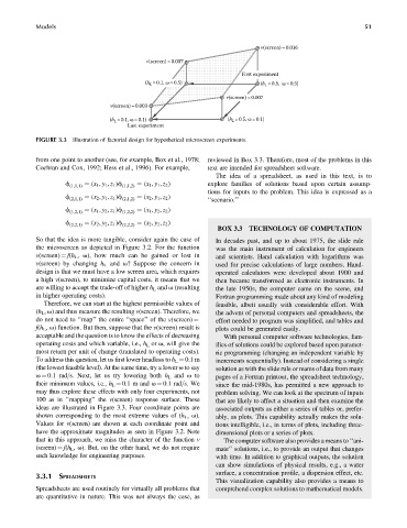
v(screen) = 0.016

v(screen) = 0.007
First experiment
(h L = 0.1, ω = 0.5) (h = 0.5, ω = 0.5)
L
v(screen) = 0.007
v(screen)=0.003

= 0.1, ω = 0.1) = 0.5, ω = 0.1)
(h L (h L
Last experiment
FIGURE 3.3 Illustration of factorial design for hypothetical microscreen experiments.

from one point to another (see, for example, Box et al., 1978; reviewed in Box 3.3. Therefore, most of the problems in this
Cochran and Cox, 1992; Hess et al., 1996). For example, text are intended for spreadsheet software.
The idea of a spreadsheet, as used in this text, is to
f (1,1,1) ¼ (x 1 , y 1 , z 1 )f (1,1,2) ¼ (x 1 , y 1 , z 2 ) explore families of solutions based upon certain assump-
tions for inputs to the problem. This idea is expressed as a
f (2,1,1) ¼ (x 2 , y 1 , z 1 )f (2,1,2) ¼ (x 2 , y 1 , z 2 ) ‘‘scenario.’’

f ¼ (x 1 , y 2 , z 1 )f ¼ (x 1 , y 2 , z 2 )
(1,2,1) (1,2,2)
f (2,2,1) ¼ (x 2 , y 2 , z 1 )f (2,2,2) ¼ (x 2 , y 2 , z 2 )
BOX 3.3 TECHNOLOGY OF COMPUTATION
So that the idea is more tangible, consider again the case of In decades past, and up to about 1975, the slide rule
the microscreen as depicted in Figure 3.2. For the function was the main instrument of calculation for engineers
v(screen) ¼ f(h L , v), how much can be gained or lost in and scientists. Hand calculation with logarithms was
v(screen) by changing h L and v? Suppose the concern in used for precise calculations of large numbers. Hand-
design is that we must have a low screen area, which requires operated calculators were developed about 1900 and
a high v(screen), to minimize capital costs, it means that we then became transformed as electronic instruments. In
are willing to accept the trade-off of higher h L and v (resulting the late 1950s, the computer came on the scene, and
in higher operating costs). Fortran programming made about any kind of modeling
Therefore, we can start at the highest permissible values of feasible, albeit usually with considerable effort. With
(h L , v) and thus measure the resulting v(screen). Therefore, we the advent of personal computers and spreadsheets, the
effort needed to program was simplified, and tables and
do not need to ‘‘map’’ the entire ‘‘space’’ of the v(screen) ¼
f(h L , v) function. But then, suppose that the v(screen) result is plots could be generated easily.
acceptable and the question is to know the effects of decreasing With personal computer software technologies, fam-
operating costs and which variable, i.e., h L or v, will give the ilies of solutions could be explored based upon paramet-
most return per unit of change (translated to operating costs). ric programming (changing an independent variable by
To address this question, let us first lower headloss to h L ¼ 0.1 m increments sequentially). Instead of considering a single
(the lowest feasible level). At the same time, try a lower v to say solution as with the slide rule or reams of data from many
v ¼ 0.1 rad=s. Next, let us try lowering both h L and v to pages of a Fortran printout, the spreadsheet technology,
their minimum values, i.e., h L ¼ 0.1 m and v ¼ 0.1 rad=s. We since the mid-1980s, has permitted a new approach to
may thus explore these effects with only four experiments, not problem solving. We can look at the spectrum of inputs
100 as in ‘‘mapping’’ the v(screen) response surface. These that are likely to affect a situation and then examine the
ideas are illustrated in Figure 3.3. Four coordinate points are associated outputs as either a series of tables or, prefer-
shown corresponding to the most extreme values of (h L , v). ably, as plots. This capability actually makes the solu-
Values for v(screen) are shown at each coordinate point and tions intelligible, i.e., in terms of plots, including three-
have the approximate magnitudes as seen in Figure 3.2. Note dimensional plots or a series of plots.
that in this approach, we miss the character of the function v The computer software also provides a means to ‘‘ani-
(screen) ¼ f(h L , v). But, on the other hand, we do not require mate’’ solutions, i.e., to provide an output that changes
such knowledge for engineering purposes. with time. In addition to graphical outputs, the solution
can show simulations of physical results, e.g., a water
surface, a concentration profile, a dispersion effect, etc.
3.3.1 SPREADSHEETS
This visualization capability also provides a means to
Spreadsheets are used routinely for virtually all problems that comprehend complex solutions to mathematical models.
are quantitative in nature. This was not always the case, as