Page 353 - gas transport in porous media

Chapter 22: Environmental Remediation of Volatile Organic Compounds
0.9 1 355
isotropic
0.8 anisotropic
0.7

0.6
c d 0.5

0.4

0.3

0.2
0.1

0
10 3 10 4 10 5 10 6 10 7 10 8
Time, seconds
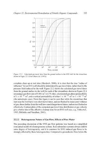
Figure 22.2. Calculated gas travel time from the ground surface to the SVE well for the streamlines
shown in Figure 22.1 (from Shan et al. (1992))

complete clean up at real sites (Murdoch, 2000), it is clear that the true “radius of
influence” for an SVE well should be determined by gas travel time, rather than by the
pressure field induced by the well. Figure 22.2 shows the calculated gas travel times
from the ground surface to the well for each of the streamlines shown in Figure 22.1
3
assuming a gas flow rate of 0.081 m /s(170 cfm), a horizontal gas phase permeability
2
2
of 1 × 10 −11 m , and a vertical permeability of either 1 × 10 −11 m or 1 × 10 −12 m 2
(the anisotropic case). From this figure it can be seen that while the streamlines that
start near the well have very short travel times, and are flushed by many pore volumes
of gas, those farther from the well have much larger travel times, and are not flushed as
effectively. Contour plots of the computed gas travel time distribution or gas velocity
give a better idea of the effective cleanup zone for an SVE well (see, e.g., Falta et al.,
1993; DiGiulio and Varadhan, 2001).

22.2.2 Heterogeneous Nature of Gas Flow, Effects of Pore Water
The preceding discussion of the SVE gas flow patterns was based on a simplified
conceptual model of a homogeneous system. Real subsurface systems always exhibit
some degree of heterogeneity, and it is common for SVE induced gas flows to be
strongly affected by these heterogeneities. Compared to groundwater flow below the