Page 272 - Geochemical Anomaly and Mineral Prospectivity Mapping in GIS

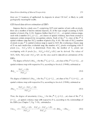
Data-Driven Modeling of Mineral Prospectivity 275

2
there are 13 locations of epithermal Au deposits in about 130 km , is likely to yield
geologically meaningful results.
GIS-based data-driven estimation of EBFs
Suppose that in a study area T, comprising N(T) total number of unit cells or pixels,
there are a number of known mineral deposits, D, of the type sought occurring in N(D)
number of pixels (Fig. 8-10). Suppose further that X i (i=1,2,…,n) spatial evidence maps,
each with a number of C ji (j=1,2,…,m) classes of spatial evidence, have been created to
th
th
represent certain prospectivity recognition criteria. Each of the j C ji class of the i X i
spatial evidence map has N(C ji) number of pixels (Fig. 8-10). The sum of N(C ji) number
th
of pixels in any i X i spatial evidence map is equal to N(T). By overlaying a binary map
of D on each multi-class evidential map, the number of C ji pixels overlapping with D
pixels [i.e., N (C ∩ D ) ] is determined. From this, the number of C ji pixels not
ji
−
overlapping with D pixels [i.e., N (C iji ) N (C ∩ D ) ] can be derived. The values of
ji
N(T), N(D), N(C ji) and N (C ∩ D ) are the ones used in data-driven estimations of the
ji
EBFs.
th
th
The degree of belief ( Bel C ji ) for the j C ji (j=1,2,…,m) class of the i X i (i=1,2,…,n)
spatial evidence map with respect to D is, according to An et al. (1994b), estimated as

N (C ∩ D )
Bel = ji . (8.4)
N (C ji )
C ji

th
th
The degree of disbelief ( Dis C ji ) for the j C ji (j=1,2,…,m) class of the i X i (i=1,2,…,n)
spatial evidence map with respect to D is, according to An et al. (1994b), estimated as

−
N (C ) N (C ∩ D )
Dis = ji ji . (8.5)
C ji
N (C ji )

th
th
Then, the degree of uncertainty (Unc C ji ) for the j C ji (j=1,2,…,m) class of the i X i
(i=1,2,…,n) spatial evidence map with respect to D is, according to the relationships of
the EBFs (see Chapter 7, Fig. 7-18), estimated as

N( C ∩ D) N( C ) − N( C ∩ D)
Unc C ji = 1 − N( ji C ) − ji N( C ) ji = 1 − Bel C ji − Dis C ji . (8.6)
ji
ji