Page 276 - Geochemical Anomaly and Mineral Prospectivity Mapping in GIS

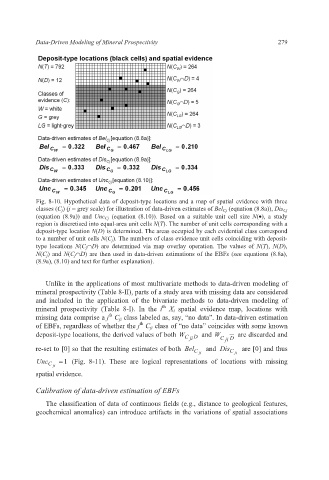
Data-Driven Modeling of Mineral Prospectivity 279

Fig. 8-10. Hypothetical data of deposit-type locations and a map of spatial evidence with three
classes (C j ) (j = grey scale) for illustration of data-driven estimates of Bel Cj (equation (8.8a)), Dis Cj
(equation (8.9a)) and Unc Cj (equation (8.10)). Based on a suitable unit cell size N(•), a study
region is discretised into equal-area unit cells N(T). The number of unit cells corresponding with a
deposit-type location N(D) is determined. The areas occupied by each evidential class correspond
to a number of unit cells N(C j ). The numbers of class evidence unit cells coinciding with deposit-
type locations N(C j ∩D) are determined via map overlay operation. The values of N(T), N(D),
N(C j ) and N(C j ∩D) are then used in data-driven estimations of the EBFs (see equations (8.8a),
(8.9a), (8.10) and text for further explanation).

Unlike in the applications of most multivariate methods to data-driven modeling of
mineral prospectivity (Table 8-II), parts of a study area with missing data are considered
and included in the application of the bivariate methods to data-driven modeling of
th
mineral prospectivity (Table 8-I). In the i X i spatial evidence map, locations with
th
missing data comprise a j C ji class labeled as, say, “no data”. In data-driven estimation
th
of EBFs, regardless of whether the j C ji class of “no data” coincides with some known
deposit-type locations, the derived values of both W C ji D and W C ji D are discarded and
re-set to [0] so that the resulting estimates of both Bel C ji and Dis C ji are [0] and thus
Unc C ji = 1 (Fig. 8-11). These are logical representations of locations with missing
spatial evidence.

Calibration of data-driven estimation of EBFs

The classification of data of continuous fields (e.g., distance to geological features,
geochemical anomalies) can introduce artifacts in the variations of spatial associations