Page 99 - Geochemistry of Oil Field Waters

EMISSION SPECTROMETRY 87

-
20-

- 40-
z
P -
v)
z -

I I I 1 1 1 ,
0
RELATIVE INTENSITY

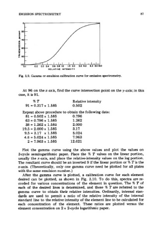
Fig. 3.9. Gamma or emulsion calibration curve for emission spectrometry.

At 96 on the x-axis, find the curve intersection point on the y-axis; in this
case, it is 91.

%T Relative intensity
91 = 0.317 x 1.585 0.502
Repeat above procedure to obtain the following data:
81 = 0.502 x 1.585 0.796
63 = 0.796 x 1.585 1.262
38 = 1.262 x 1.585 2.000
19.5 = 2.000 x 1.585 3.17
9.5 = 3.17 x 1.585 5.024
4.6 = 5.024 x 1.585 7.963
2 = 7.963 x 1.585 12.621

Plot the gamma curve using the above values and plot the values on
3-cycle semilogarithmic paper. Place the 7% T values on the linear portion,
usually the x-axis, and place the relative-intensity values on the log portion.
The resultant curve should be an inverted S if the linear portion or % T is the
x-axis. (Theoretically, only one gamma curve need be plotted for all plates
with the same emulsion number.)
After the gamma curve is plotted, a calibration curve for each element
desired can be plotted, as shown in Fig. 3.10. To do this, spectra are re-
corded for various concentrations of the element in question. The % T of
each of the desired lines is determined, and these % T are referred to the
gamma curve to obtain their relative intensities. Ordinarily, internal stan-
dards are used to permit a ratio of the relative intensity of the internal
standard line to the relative intensity of the element line to be calculated for
each concentration of the element. These ratios are plotted versus the
element concentration on 2 x 2-cycle logarithmic paper.