Page 341 - Global Tectonics

324 CHAPTER 10

1.0 1. 0
(a) (b)
α =45° α =0°
0.8 η =100 0. 8 η =100
–4 –2 0 2 4 –4 –2 0 2 4
0.6 0. 6
-1
0.4 -3 0. 4 -2 2
1
0.2 -2 4 0. 2 -3 3
2 -1
3 1
Distance x 10 km 1.0 (c) 1. 0 (d) α
4 0.0 0.0 0.2 0. 4 0.6 0. 8 1.0 0. 0 0. 0 0 .2 0. 4 0 .6 0. 8 1.0

α
=0°
=3
0.8
–4 –2 0 2 4 η =3 0. 8 –4 –2 0 2 4 η =45°
0.6 0. 6
-1
0.4 0. 4 -2
-2 2 -1
3
0.2 -4 4 3 0. 2
-4
1 1
-3
0.0 0. 0 -3 2
0.0 0.2 0.4 0.6 0.8 1.0 0.0 0.2 0.4 0.6 0.8 1.0
Distance x 10 km
4

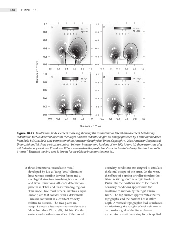
Figure 10.25 Results from finite element modeling showing the instantaneous lateral displacement field during

indentation for two different indentor rheologies and two indentor angles (a) (image provided by J. Robl and modified

from Robl & Stüwe, 2005a, by permission of the American Geophysical Union. Copyright © 2005 American Geophysical
Union). (a) and (b) show a viscosity contrast between indentor and foreland of h = 100; (c) and (d) show a contrast of h
= 3. Indentor angles of a = 0° and a = 45° are represented. Grayscale bar shows horizontal velocity. Contour interval is
−1
1 mm a . Eastward moving area is largest for the oblique indentor shown in (a).

A three-dimensional viscoelastic model boundary conditions are assigned to simulate
developed by Liu & Yang (2003) illustrates the lateral escape of the crust. On the west,
how various possible driving forces and a the effects of a spring or roller simulate the
rheological structure involving both vertical lateral resisting force of a rigid block in
and lateral variations infl uence deformation Pamir. On the northern side of the model
patterns in Tibet and its surrounding regions. boundary conditions approximate the
This model, like most others, involves a rigid resistance to motion by the rigid Tarim
Indian plate that collides with a deformable Basin. The top surface approximates the real
Eurasian continent at a constant velocity topography and the bottom lies at 70 km
relative to Eurasia. The two plates are depth. A vertical topographic load is included
coupled across a fault zone that simulates the by calculating the weight of rock columns in
Main Boundary Thrust (Fig. 10.26a). On the each surface grid of the fi nite element
eastern and southeastern sides of the model, model. An isostatic restoring force is applied