Page 183 - Glucose Monitoring Devices

The Bayesian approach applied to the calibration problem 185

BG-to-IG Calibration
kinetics function

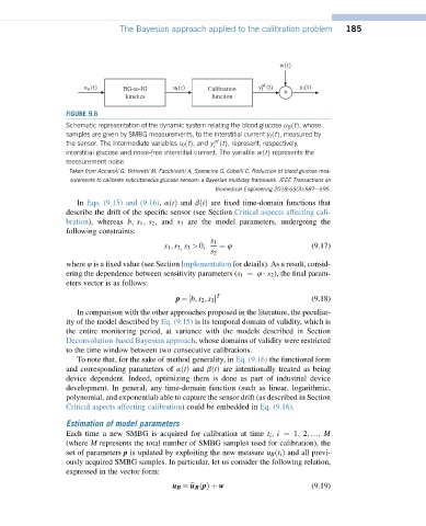
FIGURE 9.6
Schematic representation of the dynamic system relating the blood glucose u B ðtÞ, whose
samples are given by SMBG measurements, to the interstitial current y I ðtÞ, measured by
nf
the sensor. The intermediate variables u I ðtÞ, and y ðtÞ, represent, respectively,
I
interstitial glucose and noise-free interstitial current. The variable wðtÞ represents the
measurement noise.
Taken from Acciaroli G, Vettoretti M, Facchinetti A, Sparacino G, Cobelli C. Reduction of blood glucose mea-
surements to calibrate subcutaneous glucose sensors: a Bayesian multiday framework. IEEE Transactions on
Biomedical Engineering 2018;65(3):587e595.
In Eqs. (9.15) and (9.16), aðtÞ and bðtÞ are fixed time-domain functions that
describe the drift of the specific sensor (see Section Critical aspects affecting cali-
bration), whereas b; s 1 ; s 2 ; and s 3 are the model parameters, undergoing the
following constraints:
s 1
s 1 ; s 2; s 3 > 0; ¼ 4 (9.17)
s 2
where 4 is a fixed value (see Section Implementation for details). As a result, consid-
ering the dependence between sensitivity parameters (s 1 ¼ 4$ s 2 ), the final param-
eters vector is as follows:
T
p ¼½b; s 2 ; s 3 Š (9.18)
In comparison with the other approaches proposed in the literature, the peculiar-
ity of the model described by Eq. (9.15) is its temporal domain of validity, which is
the entire monitoring period, at variance with the models described in Section
Deconvolution-based Bayesian approach, whose domains of validity were restricted
to the time window between two consecutive calibrations.
To note that, for the sake of method generality, in Eq. (9.16) the functional form
and corresponding parameters of aðtÞ and bðtÞ are intentionally treated as being
device dependent. Indeed, optimizing them is done as part of industrial device
development. In general, any time-domain function (such as linear, logarithmic,
polynomial, and exponential) able to capture the sensor drift (as described in Section
Critical aspects affecting calibration) could be embedded in Eq. (9.16).
Estimation of model parameters
Each time a new SMBG is acquired for calibration at time t i ; i ¼ 1; 2; .; M
(where M represents the total number of SMBG samples used for calibration), the
set of parameters p is updated by exploiting the new measure u B ðt i Þ and all previ-
ously acquired SMBG samples. In particular, let us consider the following relation,
expressed in the vector form:
u B ¼ b u B ðpÞþ w (9.19)