Page 185 - Glucose Monitoring Devices

The Bayesian approach applied to the calibration problem 187

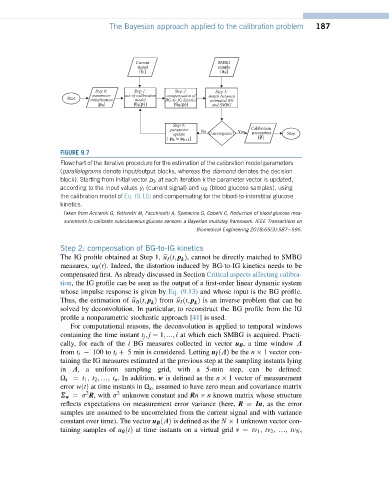
FIGURE 9.7
Flowchart of the iterative procedure for the estimation of the calibration model parameters
(parallelograms denote input/output blocks, whereas the diamond denotes the decision
block). Starting from initial vector p 0 , at each iteration k the parameter vector is updated,
according to the input values y I (current signal) and u B (blood glucose samples), using
the calibration model of Eq. (9.15) and compensating for the blood-to-interstitial glucose
kinetics.
Taken from Acciaroli G, Vettoretti M, Facchinetti A, Sparacino G, Cobelli C. Reduction of blood glucose mea-
surements to calibrate subcutaneous glucose sensors: a Bayesian multiday framework. IEEE Transactions on
Biomedical Engineering 2018;65(3):587e595.

Step 2: compensation of BG-to-IG kinetics
The IG profile obtained at Step 1, b u I ðt; p Þ, cannot be directly matched to SMBG
k
measures, u B ðtÞ. Indeed, the distortion induced by BG-to-IG kinetics needs to be
compensated first. As already discussed in Section Critical aspects affecting calibra-
tion, the IG profile can be seen as the output of a first-order linear dynamic system
whose impulse response is given by Eq. (9.13) and whose input is the BG profile.
Thus, the estimation of b u B ðt; p Þ from b u I ðt; p Þ is an inverse problem that can be
k
k
solved by deconvolution. In particular, to reconstruct the BG profile from the IG
profile a nonparametric stochastic approach [41] is used.
For computational reasons, the deconvolution is applied to temporal windows
containing the time instant t j ; j ¼ 1; :::; i at which each SMBG is acquired. Practi-
cally, for each of the i BG measures collected in vector u B , a time window L
from t i 100 to t i þ 5 min is considered. Letting u I ðLÞ be the n 1 vector con-
taining the IG measures estimated at the previous step at the sampling instants lying
in L; a uniform sampling grid, with a 5-min step, can be defined:
U s ¼ t 1 ; t 2 ; .; t n . In addition, w is defined as the n 1 vector of measurement
error wðtÞ at time instants in U s , assumed to have zero mean and covariance matrix
2
2
S w ¼ s R, with s unknown constant and Rn n known matrix whose structure
reflects expectations on measurement error variance (here, R ¼ In, as the error
samples are assumed to be uncorrelated from the current signal and with variance
constant over time). The vector u B ðLÞ is defined as the N 1 unknown vector con-
taining samples of u B ðtÞ at time instants on a virtual grid v ¼ tv 1 ; tv 2 ; .; tv N ,