Page 188 - Glucose Monitoring Devices

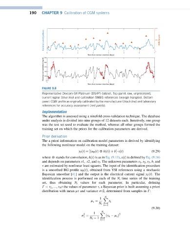
190 CHAPTER 9 Calibration of CGM systems

FIGURE 9.8
Representative Dexcom G4 Platinum (DG4P) dataset. Top panel: raw, unprocessed,
current signal (blue line) and calibration SMBG references (orange triangles). Bottom
panel: CGM profile as originally calibrated by the manufacturer (black line) and laboratory
references for accuracy assessment (red points).
Implementation
The algorithm is assessed using a ninefold cross-validation technique. The database
under analysis is divided into nine groups of 12 datasets each. Iteratively, one group
was the test set used to evaluate the method, whereas all other groups formed the
training set on which the priors for the calibration parameters are derived.

Prior derivation
The a priori information on calibration model parameters is derived by identifying
the following nonlinear model on the training dataset:

y I ðtÞ¼½ðu B ðtÞ 5 hðtÞÞ þ bŠ$sðtÞ (9.29)
where 5 stands for convolution, hðtÞ is as in Eq. (9.13), sðtÞ is defined by Eq. (9.16)
and depends on parameters s1; s2; and s 3 . The unknown parameters s 1 , s 2 , s 3 , b, and
s are estimated by nonlinear least squares. The input of the identification procedure
is a smoothed BG profile u B ðtÞ; obtained from YSI references using a stochastic
Bayesian smoother [41] and the output is the electrical current signal y I ðtÞ: The
identification process is performed on each of the N t time series of the training
set, thus obtaining N t values for each parameter. In particular, defining
G ¼ s 1 ; :::; s N t the values of parameter s, a Bayesian prior is built assuming a priori
distribution with mean ms and variance ss2, determined from samples in G:

1 X
N t
m ¼ t k
s
N t
k¼1
(9.30)
N t
1 X
2 2
s
s ¼ ðs k m Þ
s
N t 1
k¼1