Page 453 - Handbook Of Integral Equations

where the integration path is parallel to the imaginary axis of the complex plane s and the integral
is understood in the sense of the Cauchy principal value.
Formula (2) holds for continuous functions. If f(x)hasa(finite) jump discontinuity at a point

1
x = x 0 > 0, then the left-hand side of (2) is equal to f(x 0 – 0) + f(x 0 +0) at this point (for x 0 =0,
2
the first term in the square brackets must be omitted).
For brevity, we rewrite formula (2) in the form
–1 ˆ –1 ˆ
f(x)= M {f(s)}, or f(x)= M {f(s), x}.

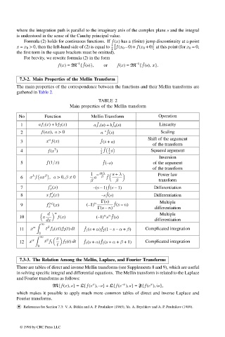
7.3-2. Main Properties of the Mellin Transform
The main properties of the correspondence between the functions and their Mellin transforms are
gathered in Table 2.
TABLE 2
Main properties of the Mellin transform

No Function Mellin Transform Operation
ˆ
ˆ
1 af 1 (x)+ bf 2 (x) af 1 (s)+ bf 2 (s) Linearity
–s ˆ
2 f(ax), a >0 a f(s) Scaling
a
ˆ
3 x f(x) f(s + a) Shift of the argument
of the transform

2
f
4 f(x ) 1 ˆ 1 s Squared argument
2 2
Inversion
ˆ
5 f(1/x) f(–s) of the argument
of the transform

β 1 – s+λ s + λ
Power law
λ
6 x f ax , a >0, β ≠ 0 a β ˆ
f
β β transform
ˆ

7 f (x) –(s – 1)f(s – 1) Differentiation
x
ˆ

8 xf (x) –sf(s) Differentiation
x
Γ(s) Multiple
ˆ
n
9 f x (n) (x) (–1) f(s – n)
Γ(s – n) differentiation
d
n Multiple
n n ˆ
10 x f(x) (–1) s f(s)
dx differentiation

∞
β
ˆ
ˆ
11 x α t f 1 (xt)f 2 (t) dt f 1 (s + α)f 2 (1 – s – α + β) Complicated integration
0

∞
x
β
ˆ
ˆ
12 x α t f 1 f 2 (t) dt f 1 (s + α)f 2 (s + α + β +1) Complicated integration
0 t
7.3-3. The Relation Among the Mellin, Laplace, and Fourier Transforms
There are tables of direct and inverse Mellin transforms (see Supplements 8 and 9), which are useful
in solving specific integral and differential equations. The Mellin transform is related to the Laplace
and Fourier transforms as follows:
x –x x
M{f(x), s} = L{f(e ), –s} + L{f(e ), s} = F{f(e ), is},
which makes it possible to apply much more common tables of direct and inverse Laplace and
Fourier transforms.
•
References for Section 7.3: V. A. Ditkin and A. P. Prudnikov (1965), Yu. A. Brychkov and A. P. Prudnikov (1989).
© 1998 by CRC Press LLC
© 1998 by CRC Press LLC
Page 434