Page 692 - Handbook Of Integral Equations

We see that the rate of convergence of the iteration process performed by the Newton–Kantorovich method is significantly
higher than that performed by the method of successive approximations (see Example 2 in Subsection 14.4-4).
To estimate the rate of convergence of the performed iteration process, we can compare the above results with the
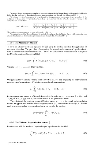
realization of the modified Newton–Kantorovich method. In connection with the latter, for the above versions of the
approximations we can obtain

k 0 k 1 k 2 k 3 k 4 k 5 k 6 k 7 k 8 ...
y n(x)=1 + k nx; .
0 0.25 0.69 0.60 0.51 0.44 0.38 0.36 0.345 ...
The iteration process converges to the exact solution y(x)=1 + 1 x.
3
We see that the modified Newton–Kantorovich method is less efficient than the Newton–Kantorovich method, but more
efficient than the method of successive approximations (see Example 2 in Subsection 14.4-4).

14.3-6. The Quadrature Method
To solve an arbitrary nonlinear equation, we can apply the method based on the application of
quadrature formulas. The procedure of composing the approximating system of equations is the
same as in the linear case (see Subsection 11.18-1). We consider this procedure for an example of
the Urysohn equation of the second kind:

b

y(x) – K x, t, y(t) dt = f(x), a ≤ x ≤ b. (41)
a
We set x = x i (i =1, ... , n). Then we obtain

b

y(x i ) – K x i , t, y(t) dt = f(x i ). i =1, ... , n, (42)
a
On applying the quadrature formula from Subsection 11.18-1 and neglecting the approximation
error, we transform relations (42) into the system of nonlinear equations

n

y i – A j K ij (y j )= f i , i =1, ... , n, (43)
j=1

for the approximate values y i of the solution y(x) at the nodes x 1 , ... , x n , where f i = f(x i ) and
K ij (y j )= K(x i , t j , y j ), and A j are the coefficients of the quadrature formula.
The solution of the nonlinear system (43) gives values y 1 , ... , y n for which by interpolation
we find an approximate solution of the integral equation (41) on the entire interval [a, b]. For the
analytic expression of an approximate solution, we can take the function

n

˜ y(x)= f(x)+ A j K(x, x j , y j ). (44)
j=1

14.3-7. The Tikhonov Regularization Method

In connection with the nonlinear Urysohn integral equation of the first kind

b

K x, t, y(t) dt = f(x), c ≤ x ≤ d, (45)
a

© 1998 by CRC Press LLC

© 1998 by CRC Press LLC
Page 675