Page 417 - Handbook of Electrical Engineering

406 HANDBOOK OF ELECTRICAL ENGINEERING

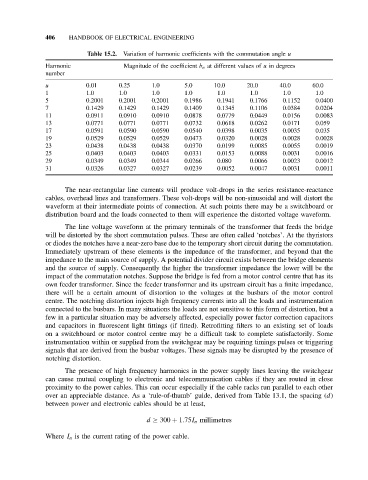
Table 15.2. Variation of harmonic coefficients with the commutation angle u

Harmonic Magnitude of the coefficient b n at different values of u in degrees
number
u 0.01 0.25 1.0 5.0 10.0 20.0 40.0 60.0
1 1.0 1.0 1.0 1.0 1.0 1.0 1.0 1.0
5 0.2001 0.2001 0.2001 0.1986 0.1941 0.1766 0.1152 0.0400
7 0.1429 0.1429 0.1429 0.1409 0.1345 0.1106 0.0384 0.0204
11 0.0911 0.0910 0.0910 0.0878 0.0779 0.0449 0.0156 0.0083
13 0.0771 0.0771 0.0771 0.0732 0.0618 0.0262 0.0171 0.059
17 0.0591 0.0590 0.0590 0.0540 0.0398 0.0035 0.0035 0.035
19 0.0529 0.0529 0.0529 0.0473 0.0320 0.0028 0.0028 0.0028
23 0.0438 0.0438 0.0438 0.0370 0.0199 0.0085 0.0055 0.0019
25 0.0403 0.0403 0.0403 0.0331 0.0153 0.0088 0.0031 0.0016
29 0.0349 0.0349 0.0344 0.0266 0.080 0.0066 0.0023 0.0012
31 0.0326 0.0327 0.0327 0.0239 0.0052 0.0047 0.0031 0.0011

The near-rectangular line currents will produce volt-drops in the series resistance-reactance
cables, overhead lines and transformers. These volt-drops will be non-sinusoidal and will distort the
waveform at their intermediate points of connection. At such points there may be a switchboard or
distribution board and the loads connected to them will experience the distorted voltage waveform.

The line voltage waveform at the primary terminals of the transformer that feeds the bridge
will be distorted by the short commutation pulses. These are often called ‘notches’. At the thyristors
or diodes the notches have a near-zero base due to the temporary short circuit during the commutation.
Immediately upstream of these elements is the impedance of the transformer, and beyond that the
impedance to the main source of supply. A potential divider circuit exists between the bridge elements
and the source of supply. Consequently the higher the transformer impedance the lower will be the
impact of the commutation notches. Suppose the bridge is fed from a motor control centre that has its
own feeder transformer. Since the feeder transformer and its upstream circuit has a finite impedance,
there will be a certain amount of distortion to the voltages at the busbars of the motor control
centre. The notching distortion injects high frequency currents into all the loads and instrumentation
connected to the busbars. In many situations the loads are not sensitive to this form of distortion, but a
few in a particular situation may be adversely affected, especially power factor correction capacitors
and capacitors in fluorescent light fittings (if fitted). Retrofitting filters to an existing set of loads
on a switchboard or motor control centre may be a difficult task to complete satisfactorily. Some
instrumentation within or supplied from the switchgear may be requiring timings pulses or triggering
signals that are derived from the busbar voltages. These signals may be disrupted by the presence of
notching distortion.
The presence of high frequency harmonics in the power supply lines leaving the switchgear
can cause mutual coupling to electronic and telecommunication cables if they are routed in close
proximity to the power cables. This can occur especially if the cable racks run parallel to each other
over an appreciable distance. As a ‘rule-of-thumb’ guide, derived from Table 13.1, the spacing (d)
between power and electronic cables should be at least,

d ≥ 300 + 1.75I n millimetres

Where I n is the current rating of the power cable.