Page 507 - Handbook of Electrical Engineering

GENERALISED THEORY OF ELECTRICAL MACHINES 497

primary are transformed to their equivalent two-phase variables. These transformations are detailed
in References 3, 5 and 6 for example. The result is a transposition of the rows in the voltage-current
equation (20.24) and the insertion of suffices 1 and 2, 1 for the primary and 2 for the secondary (as
with static transformers). Equation (20.24) becomes:-

     
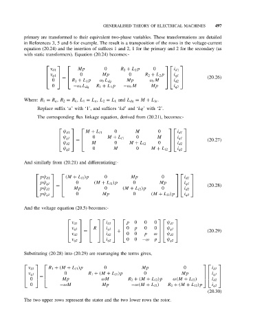
Mp 0 R 2 + L 2 p 0
v d1 i d1
v 0 Mp 0 R 2 + L 2 p i
     
= (20.26)
 q1     q1 
 R 1 + L 1 p
ω r L dq
 0  Mp ω r M   i d2 
0 −ω r L dq R 1 + L 1 p −ω r M Mp i q2
Where: R 1 = R a , R 2 = R k , L 1 = L a , L 2 = L k and L dq = M + L la .
Replace suffix ‘a’ with ‘1’, and suffices ‘kd’and ‘kq’ with ‘2’.
The corresponding flux linkage equation, derived from (20.21), becomes:-

     
0 M 0
ψ d1 M + L l1 i d1
0 0 M i
   M + L l1   
 ψ q1  =    q1  (20.27)
 ψ d2   M 0 M + L l2 0   i d2 
0 M 0
ψ q2 M + L l2 i q2
And similarly from (20.21) and differentiating:-

     
pψ d1 (M + L l1 )p 0 Mp 0 i d1
0 0
   (M + L l1 )p Mp   i 
 pψ q1  =    q1  (20.28)
 pψ d2   Mp 0 (M + L l2 )p 0   i d2 
0 Mp 0 (M + L l2 )p
pψ q2 i q2
And the voltage equation (20.5) becomes:-

         
v d1 i d1 p 0 0 0 ψ d1
 v   R   i   0 p 0 0   
 q1  =    q1  +    ψ q1  (20.29)
 v d2     i d2   0 0 p ω   ψ d2 
0 0 −ω p
v q2 i q2 ψ q2
Substituting (20.28) into (20.29) are rearranging the terms gives,

     
R 1 + (M + L l1 )p 0 Mp 0
v d1 i d1
 v   0 R 1 + (M + L l1 )p 0 Mp   i 
=
 q1     q1 
Mp ωM R 2 + (M + L l2 )p ω(M + L l2 )   i d2
 0   
0 −ωM Mp −ω(M + L l2 ) R 2 + (M + L l2 )p i q2
(20.30)
The two upper rows represent the stator and the two lower rows the rotor.