Page 508 - Handbook of Electrical Engineering

498 HANDBOOK OF ELECTRICAL ENGINEERING

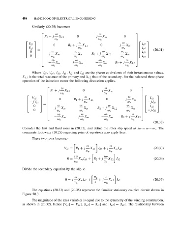
Similarly (20.25) becomes:

ω ω
 
R 1 + j X L1 0 j X m 0
 ω n ω n 
ω ω

    
V d1  0 0  I d1
 R 1 + j X L1 j X m 
   ω n ω n   I 
= (20.31)
V q1 
    q1 
 ω ω r ω ω r   I d2
j R 2 + j
 0  
 X m X m X L2 X m 
0  ω n ω n ω n ω n  I q2
 
 ω r ω ω r ω 
− X m j X m − X m R 2 + j X L2
ω n ω n ω n ω n
Where V d1 , V q1 , I d1 , I q1 , I d2 and I q2 are the phasor equivalents of their instantaneous values,
X L1 is the total reactance of the primary and X L2 that of the secondary. For the balanced three-phase
operation of the induction motor the following discussion applies.
ω ω
 
R 1 + j X L1 0 j X m 0
 ω n ω n 
ω ω

    
V d1  0 0  I d1
 R 1 + j X L1 j X m 
   ω n ω n   
 −jV d1  =    −jI d1 
0 ω ω   I d2
   ω r ω r 
 j X m X m R 2 + j X L2 X m 
0  ω n ω n ω n ω n  −jI d2
 
 ω r ω ω r ω 
− X m j X m − X m R 2 + j X L2
ω n ω n ω n ω n
(20.32)
Consider the first and third rows in (20.32), and define the rotor slip speed as sω = ω − ω r .The
comments following (20.25) regarding pairs of equations also apply here.
These two rows become:-

ω ω
V d1 = R 1 + j X L1 I d1 + j X m I d2 (20.33)
ω n ω n

sω sω
0 = X m I d1 + R 2 + j X L2 I d2 (20.34)
ω n ω n
Divide the secondary equation by the slip s:-
ω
R 2 ω
0 = j X m I d1 + + j X L2 I d2 (20.35)
ω n s ω n
The equations (20.33) and (20.35) represent the familiar stationary coupled circuit shown in
Figure 20.3.
The magnitude of the axes variables is equal due to the symmetry of the winding construction,
as shown in (20.32). Hence |V q1 |=|V d1 |, |I q1 |=|I d1 | and |I q2 |=|I d2 |. The relationship between