Page 216 -

5.2. MATRICES AND DETERMINANTS 183

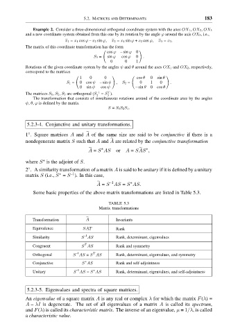
Example 2. Consider a three-dimensional orthogonal coordinate system with the axes OX 1, OX 2, OX 3
and a new coordinate system obtained from this one by its rotation by the angle ϕ around the axis OX 3, i.e.,
2 x 1 = x 1 cos ϕ – x 2 sin ϕ, 2 x 2 = x 1 sin ϕ + x 2 cos ϕ, 2 x 3 = x 3.
The matrix of this coordinate transformation has the form
( 0 )
cos ϕ –sin ϕ
S 3 = sin ϕ cos ϕ 0 .
0 0 1
Rotations of the given coordinate system by the angles ψ and θ around the axes OX 1 and OX 2, respectively,
correspond to the matrices
( 1 0 0 ) ( cos θ 0 sin θ )
S 1 = 0 cos ψ –sin ψ , S 2 = 0 1 0 .
0 sin ψ cos ψ –sin θ 0 cos θ
–1
T
The matrices S 1, S 2, S 3 are orthogonal (S j = S j ).
The transformation that consists of simultaneous rotations around of the coordinate axes by the angles
ψ, θ, ϕ is defined by the matrix
S = S 3S 2S 1.

5.2.3-4. Conjunctive and unitary transformations.
1 . Square matrices A and A of the same size are said to be conjunctive if there is a
◦
2
nondegenerate matrix S such that A and A are related by the conjunctive transformation
2
∗
∗
A = S AS or A = SAS ,
2
2
where S is the adjoint of S.
∗
2 . A similarity transformation of a matrix A is said to be unitary if it is defined by a unitary
◦
–1
∗
matrix S (i.e., S = S ). In this case,
–1
A = S AS = S AS.
∗
2
Some basic properties of the above matrix transformations are listed in Table 5.3.
TABLE 5.3
Matrix transformations
Transformation A Invariants
2
Equivalence SAT Rank
–1
Similarity S AS Rank, determinant, eigenvalues
T
Congruent S AS Rank and symmetry
–1
T
Orthogonal S AS = S AS Rank, determinant, eigenvalues, and symmetry
∗
Conjunctive S AS Rank and self-adjointness
–1
∗
Unitary S AS = S AS Rank, determinant, eigenvalues, and self-adjointness
5.2.3-5. Eigenvalues and spectra of square matrices.
An eigenvalue of a square matrix A is any real or complex λ for which the matrix F(λ) ≡
A – λI is degenerate. The set of all eigenvalues of a matrix A is called its spectrum,
and F(λ) is called its characteristic matrix. The inverse of an eigenvalue, μ = 1/λ, is called
a characteristic value.