Page 219 -

186 ALGEBRA

Suppose that the spectra of matrices A and B consist of eigenvalues λ j and μ k , respec-
tively. Then the spectrum of the Kronecker product A ⊗ B is the set of all products λ j μ k .
The spectrum of the direct sum of matrices A = A 1 ⊕ ... ⊕ A n is the union of the spectra of
the matrices A 1 , ... , A n . The algebraic multiplicities of the same eigenvalues of matrices
A 1 , ... , A n are summed.
Regarding bounds for eigenvalues see Paragraph 5.6.3-4.

5.2.3-9. Cayley–Hamilton theorem. Sylvester theorem.
CAYLEY–HAMILTON THEOREM. Each square matrix A satisfies its own characteristic equa-
tion; i.e., f A (A)= 0.
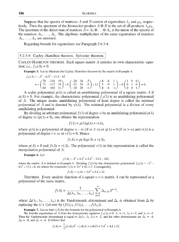
Example 5. Let us illustrate the Cayley–Hamilton theorem by the matrix in Example 4:
3 2
f A(A)= –A – 6A – 11A – 6I
70 –116 19 –20 34 –5 4 –8 1 100
( ) ( ) ( ) ( )
=– 71 –117 19 – 6 –21 35 –5 – 11 5 –9 1 – 6 010 = 0.
64 –102 11 –18 28 –1 4 –6 –1 001
A scalar polynomial p(λ) is called an annihilating polynomial of a square matrix A if
p(A)= 0. For example, the characteristic polynomial f A (λ) is an annihilating polynomial
of A. The unique monic annihilating polynomial of least degree is called the minimal
polynomial of A and is denoted by ψ(λ). The minimal polynomial is a divisor of every
annihilating polynomial.
By dividing an arbitrary polynomial f(λ)of degree n by an annihilating polynomial p(λ)
of degree m (p(λ) ≠ 0), one obtains the representation

f(λ)= p(λ)q(λ)+ r(λ),
where q(λ) is a polynomial of degree n – m (if m ≤ n)or q(λ)= 0 (if m > n)and r(λ)isa
polynomial of degree l < m or r(λ)= 0. Hence
f(A)= p(A)q(A)+ r(A),

where p(A)= 0 and f(A)= r(A). The polynomial r(λ) in this representation is called the
interpolation polynomial of A.
Example 6. Let
4 3 2
f(A)= A + 4A + 2A – 12A – 10I,
3
where the matrix A is defined in Example 4. Dividing f(λ) by the characteristic polynomial f A(λ)= –λ –
2
2
6λ – 11λ – 6, we obtain the remainder r(λ)= 3λ + 4λ + 2. Consequently,
2
f(A)= r(A)= 3A + 4A + 2I.
THEOREM. Every analytic function of a square n × n matrix A can be represented as a
polynomial of the same matrix,
n
1
f(A)= Δ n–k A n–k ,
Δ(λ 1 , λ 2 , ... , λ n )
k=1
where Δ(λ 1 , λ 2 , ... , λ n ) is the Vandermonde determinant and Δ i is obtained from Δ by
replacing the (i + 1)st row by (f(λ 1 ), f(λ 2 ), ... , f(λ n )).
Example 7. Let us find r(A) by this formula for the polynomial in Example 6.
We find the eigenvalues of A from the characteristic equation f A(λ)= 0: λ 1 =–1, λ 2 =–2,and λ 3 =–3.
Then the Vandermonde determinant is equal to Δ(λ 1, λ 2, λ 3)= –2, and the other determinants are Δ 1 =–4,
Δ 2 =–8,and Δ 3 =–6. It follows that
1
2
2
f(A)= [(–6)A +(–8)A +(–4)I]= 3A + 4A + 2I.
–2