Page 230 - Handbook of Properties of Textile and Technical Fibres

Engineering properties of spider silk 205

approaches a steady state. We can deduce the following equations from Eqs. (6.23),
(6.25) and (6.17):

1 Cg Clnðt 0 Þþ Clnðs 2 Þ
Gðt 0 Þ¼ (6.27)
1 þ Cg Clnðs 2 Þ Clnðs 1 Þ

C
S R ¼ (6.28)
1 þ Clnðs 2 Þ Clnðs 1 Þ
1
GðNÞ¼ (6.29)
1 þ Clnðs 2 Þ Clnðs 1 Þ

Note that obtaining G(N) in the true sense is almost impossible. For a first approx-
imation, we may use an arbitrary value of G(t) beyond the termination time of an
experiment. As in most situations, extrapolations outside the experimental range
should be viewed with caution.
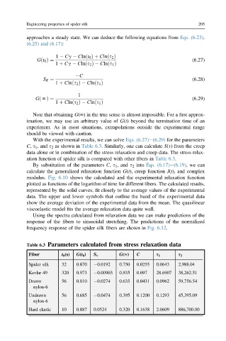
With the experimental results, we can solve Eqs. (6.27)e(6.29) for the parameters
C, s 1 , and s 2 as shown in Table 6.3. Similarly, one can calculate S(s) from the creep
data alone or in combination of the stress relaxation and creep data. The stress relax-
ation function of spider silk is compared with other fibers in Table 6.3.
By substitution of the parameters C, s 1 , and s 2 into Eqs. (6.17)e(6.19), we can
calculate the generalized relaxation function G(t), creep function J(t), and complex
modulus. Fig. 6.10 shows the calculated and the experimental relaxation function
plotted as functions of the logarithm of time for different fibers. The calculated results,
represented by the solid curves, fit closely to the average values of the experimental
data. The upper and lower symbols that outline the band of the experimental data
show the average deviation of the experimental data from the mean. The quasilinear
viscoelastic model fits the average relaxation data quite well.
Using the spectra calculated from relaxation data we can make predictions of the
response of the fibers to sinusoidal stretching. The predictions of the normalized
frequency response of the spider silk fibers are shown in Fig. 6.12.

Table 6.3 Parameters calculated from stress relaxation data
Fiber t 0 (s) G(t 0 ) S s G(N) C s 1 s 2
Spider silk 32 0.870 0.0192 0.750 0.0255 0.0643 2,988.04
Kevlar 49 320 0.973 0.00903 0.935 0.097 28.6907 38,262.51
Drawn 56 0.810 0.0274 0.635 0.0431 0.0962 59,756.54
nylon-6
Undrawn 56 0.685 0.0474 0.395 0.1200 0.1293 45,395.09
nylon-6
Hard elastic 10 0.887 0.0524 0.320 0.1638 2.0609 886,700.00