Page 36 - Handbook of Properties of Textile and Technical Fibres

Introduction to the science of fibers 17

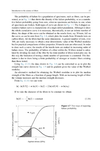
The probability of failure for a population of specimens, such as fibers, can be pre-
sented, as in Fig. 1.6 that shows the density of the failure probability, or as a cumula-
tive failure probability going from zero, when no specimens are broken, to one, when
all specimens are broken. Both types of curve are shown in Fig. 1.7. The S-shaped cu-
mulative failure curve is characteristic of a single defect population. Although to draw
the whole cumulative curve it is necessary, theoretically, to test an infinite number of
fibers, the shape of the curve can be obtained as the results from, say 30 tests, fall on
the curve, as can be seen from Fig. 1.8, which plots the results from 30 tensile tests on
carbon fibers. All the fibers had the same dimensions. A greater number of tests, over
300, are really necessary to obtain a true deterministic value of the Weibull modulus
but for practical comparisons of fiber properties 30 tensile tests are often used. In order
to draw such a curve, the results of the tensile tests are ranked in increasing order of
failure stress. The probability of failure of a fiber within the 30 fibers tested is calcu-
lated by dividing the rank of the fiber by the total number of fibers tested plus one. In
this way the limitation of testing a finite number of specimens is countered. This lim-
itation is due to there being a finite probability of stronger or weaker fibers existing
than those tested.
Using Eq. (1.13) the data shown in Fig. 1.8 can be converted so as to plot the
straight line curve shown in Fig. 1.9 and its gradient gives the value of the Weibull
modulus.
An alternative method for obtaining the Weibull modulus is to plot the median
strength of the fibers as a function of gauge length. With an increasing length of fiber
the volume increases and the median strength decreases.
From Eq. (1.11) we can write

ln½ lnð0:5ފ ¼ m lnðsÞþ lnðlÞþ 2lnðpD=4Þ m lnðs 0 Þ

If we take the diameter of the fibers to be constant we obtain

1
lnðsÞ¼ lnðlÞþ constant (1.14)
m

1 Figure 1.7 Two ways of depicting
failure probability.
P (σ)
Cumulative failure probability 0.5 g(σ) Density of failure probability (GPa -1 )
R

0
0 2 4
Applied stress (GPa)