Page 153 - Hardware Implementation of Finite-Field Arithmetic

136 Cha pte r F i v e

Exponentiation can also be computed using the binary or
“square and multiply” method given in Sec. 5.3 for OEFs. If the
function OEF_LSE_mult(a, b, c) computes the LSE-first multiplica-
tion a(x)b(x) mod f(x), with f(x) = x – c, given in Algorithm 5.11,
m
then the following algorithm implements the exponentiation given
in Algorithm 5.8 for OEFs:

Algorithm 5.12—Square-and-multiply exponentiation for OEF
for i in 0 .. m-1 loop b(i) := 0; end loop;
d := a; b(0) := 1;
for i in 0 .. m-1 loop
if k(i) = 1 then
b := OEF_LSE_mult(b,d,c);
end if;
d := OEF_LSE_mult(d,d,c);
end loop;
where the result of the exponentiation is the final value of the b(x)
polynomial, and where the multiplication and squaring operations
are both computed with the function OEF_LSE_mult given in
Algorithm 5.11. Furthermore, in Algorithm 5.12, t has been selected to
be equal to m. An executable Ada file OEF_exp.adb, including
Algorithm 5.12, is available at www.arithmetic-circuits.org.

5.5 FPGA Implementations
Several circuits described in this chapter have been implemented
within a Xilinx Spartan3 (speed grade-5) programmable devices. The
times (period, total time) are expressed in ns. The parameters FFs and
LUTs represent the numbers of flip-flops and look-up tables, respec-
tively. Every slice includes two flip-flops and two look-up tables. All
the source files are available at www.arithmetic- circuits.org.

5.5.1 Adders of Polynomials mod p
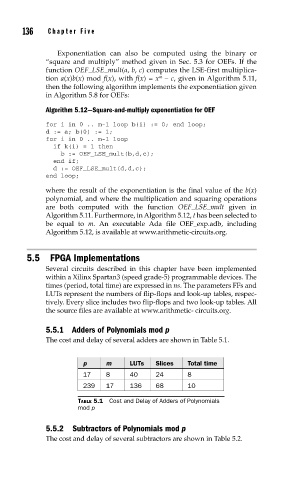
The cost and delay of several adders are shown in Table 5.1.

p m LUTs Slices Total time
17 8 40 24 8
239 17 136 68 10

TABLE 5.1 Cost and Delay of Adders of Polynomials
mod p

5.5.2 Subtractors of Polynomials mod p
The cost and delay of several subtractors are shown in Table 5.2.