Page 190 - Hardware Implementation of Finite-Field Arithmetic

m
Operations over GF (2 )—Polynomial Bases 171

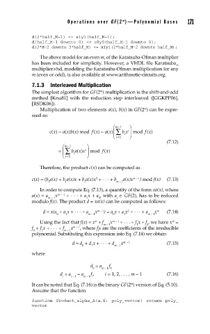
d(3*half_M-1) <= x1y1(half_M-1);
d(half_M-1 downto 0) <= x0y0(half_M-1 downto 0);
d(2*M-2 downto 3*half_M) <= x1y1(2*half_M-2 downto half_M);

The above model for an even m, of the Karatsuba-Ofman multiplier
has been included for simplicity. However, a VHDL file Karatsuba_
multiplier.vhd, modeling the Karatsuba-Ofman multiplication for any
m (even or odd), is also available at www.arithmetic-circuits.org.

7.1.3 Interleaved Multiplication
m
The simple st algorithm for GF(2 ) multiplication is the shift-and-add
method [Knu81] with the reduction step interleaved ([GGKPP06],
[RSDK06]).
m
Multiplication of two elements a(x), b(x) in GF(2 ) can be expre-
ssed as:
⎛ m−1 ⎞
c x () = ax bx () mod f x () = ax () ⎜∑ b x i mood fx()
()
i ⎟
i ⎝ =0 ⎠
(7.12)
⎛ m−1 ⎞
= ⎜∑ ba x x i ⎟ mod f x()
()
i
i ⎝ =0 ⎠
Therefore, the product c(x) can be computed as
2
c(x) = (b a(x) + b a(x)x + b a(x)x + . . . + b a(x)x m - 1 ) mod f(x) (7.13)
0 1 2 m - 1
In order to compute Eq. (7.13), a quantity of the form xa(x), where
a(x) = a x m − 1 + . . . + a x + a , with a ∈ GF(2), has to be reduced
m − 1 1 0 i
modulo f(x). The product d = xa(x) can be computed as follows:
2
d = x(a + a x + . . . + a x m - 1 ) = a x+ a x + . . . + a x m (7.14)
0 1 m − 1 0 1 m - 1
m
m
Using the fact that f(x) = x + f x m − 1 + . . . + f x + f , we have x =
m − 1 1 0
f + f x + . . . + f x m − 1 , where fs are the coefficients of the irreducible
0 1 m − 1 i
polynomial. Substituting this expression into Eq. (7.14) we obtain
d = d + d x + . . . + d x m - 1 (7.15)
0 1 m − 1
where
d = a f
0 m − 1 0
d = a + a f , i = 1, 2, . . . , m – 1 (7.16)
i i - 1 m - 1 i
m
It can be noted that Eq. (7.16) is the binary GF(2 ) version of Eq. (5.10).
Assume that the function
function Product_alpha_A(a,f: poly_vector) return poly_
vector