Page 236 - Hardware Implementation of Finite-Field Arithmetic

216 Cha pte r Se v e n

If the product of two field elements A and B is computed as given
T
in Eq. (7.29), that is, C = D + P E, and if the vectors E are defined as
(i)
E = e ( i () e , i () , ... e , i () ) = P T E, then the product C can be written as
i ()
T
0 1 m−1 i
C = D + E + E + E + . . . + E (t) (7.51)
(0)
(1)
(2)
Assuming that k ≠ 1 and using P as shown in Fig. 7.10a, the
1 0
(0)
elements of E in Eq. (7.51) are given as follows [RH04]:
⎧ e + e + + e + e ; 0 ≤ j ≤ k − 2
+
−
−
+
−
+
⎪ j j mk t j mk 2 j mk 1 1
⎪ e e + e j m k + + e j m k ; k − ≤ ≤1 j k − 2
−
−
+
+
1
2
j
⎪ t 2
0
e () = ⎨ (7.52)
j e + −≤ j ≤
⎪ ⎪ j e j m− k k t ; k t−1 1 k − 2
+
t
⎪ e ; k −≤ ≤ m − 2
j
1
⎪ j t
⎩ 0 j ; = m − 1
()
By reusing the terms e s given in Eq. (7.52), the coordinates of
0
j
(i)
E , for 1 ≤ i ≤ t, can be given as
⎧ ; 00 ≤≤ k − 1
j
⎪
e j i () = ⎨ ( ) 0 i (7.53)
⎩ ⎪ e jk i ;otherwise
−
Using Eqs. (7.52) and (7.53), the coordinates of the product C
given as Eq. (7.51) can be computed as follows [RH04]:
⎧ e () ; 0 ≤≤ k − 1
0
j
⎪ j 1
1
0
⎪ e () + e ( ) ; k ≤ ≤ k − 1
j
⎪ j j 1 2
⎪
c = d + ⎨ () 0 + ( ) 1 + + t ( − ) 1 ≤ j ≤ k − (7.54)
j
j
⎪ e e j e j e j ; k t 1 t 1
−
⎪ e () 0 + e (1) + e ( ) t ; k ≤ ≤ m − 2
+
1
j
⎪ j j j t
−
+
⎪ e j 1 () + e j 2 ( ) + e ( ) t j ; j = m − 1
⎩
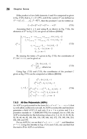
7.6.3 All-One Polynomials (AOPs)
m
An AOP is a poly nomial i n the form f(x) = x + x m − 1 + . . . + x + 1, that
is, with all its coefficients not null. An AOP is irreducible and therefore
generates a field GF(2 ) if and only if m + 1 is a prime and 2 is a
m
primitive modulo m + 1 [MBGMVY93]. For example, for m ≤ 300, the
AOP is irreducible for the following values of m: 2, 4, 10, 12, 18, 28, 36,
52, 58, 60, 66, 82, 100, 106, 130, 138, 148, 162, 172, 178, 180, 196, 210,
226, 268, and 292.
m
For an AOP f(x), we see that x = 1 + x + . . . + x m − 1 , and therefore
x m + 1 = 1. Using this identity in Eqs. (7.21) and (7.22), one can find that
the matrix P for AOPs is as follows: