Page 234 - Hardware Implementation of Finite-Field Arithmetic

214 Cha pte r Se v e n

0 s m – s m – 1
0 x x x
x x x
x x . . . x
x x x
s x
x
x
x
x
x
x
m – 2 x

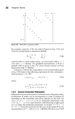
FIGURE 7.9 Matrix P for a general s-ESP.
For example, using Eq. (7.47), the matrix P given in Eqs. (7.21) and
(7.22) for multiplication is obtained as [RH04]:
⎛ I I ... I ⎞
P = ⎜ s s s ⎟ (7.48)
I
−−
⎝ ms 1 0 s +1 ⎠

where I is the j × j unity matrix and 0 is a zero matrix with m – s – 1
j s + 1
rows and s + 1 columns. The graphical representation of P for a
general s-ESP is given in Fig. 7.9, where nonzero entries of P are
represented with “x” [RH04].
Using Eq. (7.48) for the computation of the multiplication given
in Eq. (7.29) leads to the following expressions for the coordinates c
j
of the product C = D + P E
T
c = g + e 0 ≤ j ≤ m – 1 (7.49)
j j j mod s
where
−
⎧ d + e ; 0 ≤ j ≤ m s − 2
⎪
+
g = ⎨ j j s (7.50)
−− ≤
j dm s 1 j ≤ m − 1
;
⎩ ⎪ j
7.6.2 General Irreducible Polynomials
Dif ferent P matrices can be found for different irreducible polynomials.
Furthermore, P matrix can be decomposed in a sum of matrices P
i
depending on the irreducible polynomial selected for the field. Let
fx () = x + x t + ... + x + x + 1 be an irreducible polynomial, with
k
k
k
m
1
2
1 ≤ k < k < . . . < k ≤ m/2 and therefore with Hamming weight equal
1
2
t
to t + 2. Using this irreducible polynomial, we see that x = x t + ... +
k
m
x 2 + x 1 + 1. It must be noted that all the rows of the matrix P are the
k
k
representations of x m + i , with 0 ≤ i ≤ m – 2 [RH04]. Therefore, row 0 of P