Page 311 - High Power Laser Handbook

280 So l i d - S t at e La s e r s Heat-Capacity Lasers 281

3
y = m0*exp(m1 + m2*m0 + m3*m0^2 + m4*m0^3)
Value Error
2.5 m1 −0.7798 0.097168
m2 1.3777 0.30697
m3 −1.0729 0.30777
m4 0.5353 0.097912
2
Chisq 0.0017145 NA
R 0.99992 NA
M ASE − 1 1.5

1

YAG
0.5
10 × 10 × 2 cm 3
0
0 0.2 0.4 0.6 0.8 1 1.2 1.4 1.6
gL
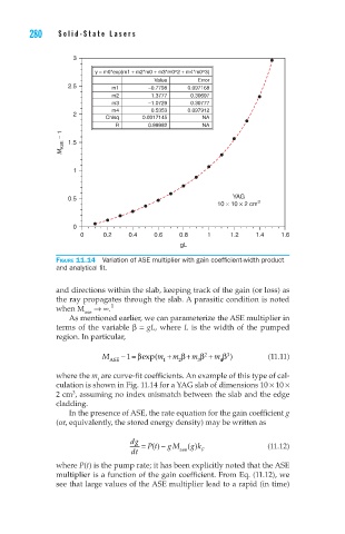
Figure 11.14 Variation of ASE multiplier with gain coefficient-width product
and analytical fit.

and directions within the slab, keeping track of the gain (or loss) as
the ray propagates through the slab. A parasitic condition is noted
when M → ∞. 1
ase
As mentioned earlier, we can parameterize the ASE multiplier in
terms of the variable b = gL, where L is the width of the pumped
region. In particular,

M −= b 1 m + m + bexp( m b 2 + m b 3 ) (11.11)
ASE 1 2 3 4
where the m are curve-fit coefficients. An example of this type of cal-
i
culation is shown in Fig. 11.14 for a YAG slab of dimensions 10 × 10 ×
2 cm , assuming no index mismatch between the slab and the edge
3
cladding.
In the presence of ASE, the rate equation for the gain coefficient g
(or, equivalently, the stored energy density) may be written as

dg = Pt − () gM () (11.12)
gk
dt ase F
where P(t) is the pump rate; it has been explicitly noted that the ASE
multiplier is a function of the gain coefficient. From Eq. (11.12), we
see that large values of the ASE multiplier lead to a rapid (in time)