Page 227 - Innovations in Intelligent Machines

220 S. Pr¨uter et al.
5.5 Calculation Time

In this experiment, the time needed to evaluate a population is measured.
The parameters vary from 1 to 3 for µ and10to30for λ. µ is denoting the
parent population size while λ is denoting the number of children. The scenario
includes four obstacles along the path. For this measurement a plus strategy
is used. All times in Table 1 are averaged measurements with a maximal error
of 0.9 ms. The timings vary because the randomly chosen genetic operators
need different times.
The result indicates that it is possible to use up to 30 offspring in one
generation. However, due to variations in calculation speed, it is saver to use
only 20 offspring.

5.6 Finding a Path in Dynamic Environments
In real-world scenarios, the obstacles as well as the robot are moving. The
movement of the obstacles starts at time step 10 and finishes at time step 30.
The robot drives with a speed of 5 pixels per time step. At the beginning, the
obstacles are positioned in a way that the robot has enough space between
them. In their end position, the robot needs to drive around them.
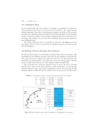
Fig. 25 shows that until the obstacles start to move, the error function
has the same value as the direct distance to the destination. As soon as the
obstacle starts to move, the robot is adjusting its path. At time step 22, the
distance between both obstacles is smaller than the robot size. At this point,

Table 1. Calculation time for one generation depending on µ and λ
µ λ =10 λ =20 λ =30
1 5.5 ms 11.2 ms 15.5 ms
2 6.5 ms 14.8 ms 20.7 ms
3 7.2 ms 14.4 ms 20.5 ms

Destination obstacle movement
700
robot Distance
600 to Des-
path tination
500
Fitness
400
300
original
robot path 200
Path change New path
needed found
100
Start 0
0 10 20 30
Generation
Fig. 25. Path planning and robot movement in a dynamic environment