Page 226 - Innovations in Intelligent Machines

Evolutionary Design of a Control Architecture for Soccer-Playing Robots 219
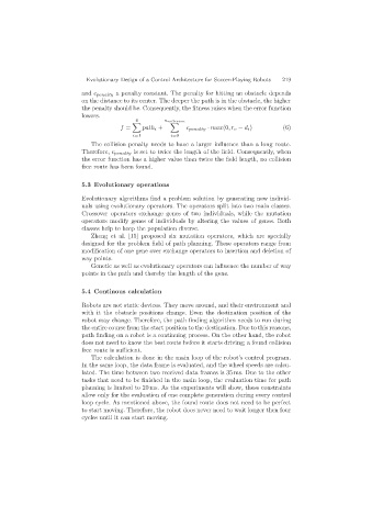
and c penalty a penalty constant. The penalty for hitting an obstacle depends
on the distance to its center. The deeper the path is in the obstacle, the higher
the penalty should be. Consequently, the fitness raises when the error function
lowers.
4 n collision

f = path i + c penalty · max(0,r o − d i ) (6)
i=1 i=0
The collision penalty needs to have a larger influence than a long route.
Therefore, c penalty is set to twice the length of the field. Consequently, when
the error function has a higher value than twice the field length, no collision
free route has been found.

5.3 Evolutionary operations

Evolutionary algorithms find a problem solution by generating new individ-
uals using evolutionary operators. The operators split into two main classes.
Crossover operators exchange genes of two individuals, while the mutation
operators modify genes of individuals by altering the values of genes. Both
classes help to keep the population diverse.
Zheng et al. [15] proposed six mutation operators, which are specially
designed for the problem field of path planning. These operators range from
modification of one gene over exchange operators to insertion and deletion of
way points.
Genetic as well as evolutionary operators can influence the number of way
points in the path and thereby the length of the gene.

5.4 Continous calculation
Robots are not static devices. They move around, and their environment and
with it the obstacle positions change. Even the destination position of the
robot may change. Therefore, the path finding algorithm needs to run during
the entire course from the start position to the destination. Due to this reasons,
path finding on a robot is a continuing process. On the other hand, the robot
does not need to know the best route before it starts driving; a found collision
free route is sufficient.
The calculation is done in the main loop of the robot’s control program.
In the same loop, the data frame is evaluated, and the wheel speeds are calcu-
lated. The time between two received data frames is 35 ms. Due to the other
tasks that need to be finished in the main loop, the evaluation time for path
planning is limited to 20 ms. As the experiments will show, these constraints
allow only for the evaluation of one complete generation during every control
loop cycle. As mentioned above, the found route does not need to be perfect
to start moving. Therefore, the robot does never need to wait longer then four
cycles until it can start moving.