Page 222 - Innovations in Intelligent Machines

Evolutionary Design of a Control Architecture for Soccer-Playing Robots 215

target
angle
target position

target y offset angle

offset y
global angle

target x offset x
robot

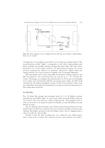
Fig. 19. And example of the configuration for the slip and friction compensation.
See text for details

corresponds to the position as provided by the image processing system. The
second position called “offset”, corresponds to the robot’s true position and
hence includes the traveled distance during the time delay. The third robot
symbolizes the robot’s target position. As mentioned previously, the neural
network estimates the robot’s true positions (labeled by “offset”) from the
target position, the robot’s previous position, and its traveled distances.
All experiments were done using 400 pre-selected training patterns and
800 test patterns. The initial learning rate was set to η =0.1. During the
course of learning, the learning rate was increased by 2% in case of decreasing
error values and decreased by 50% for increasing error values. In 10% of all
experiments, the back-propagation became ‘stuck’ in local optima. These runs
were discarded. Learning was terminated, if no improvement was obtained over
100 consecutive iterations.

4.4 Results

Fig. 20 shows the average and maximal error for 3 to 50 hidden neurons
organized in one hidden layer. It can be seen that above 20 hidden neurons,
the network does not yield any further improvement. This suggests that in
order to account for the limited resources available, at most 20 hidden neurons
should be used.
Fig. 21 and Fig. 22 summarize some results achieved by networks with two
hidden layers. Preliminary experiments have focused on finding a suitable ratio
between the hidden neurons in the two hidden layers. Fig. 21 suggests that a
ratio 3:1 yield the best results.
Similar to Fig. 20, Fig. 22 shows the error values for two hidden layers
with a ratio of 3:1 neurons. The numbers on the x-axis indicate the number