Page 218 - Innovations in Intelligent Machines

Evolutionary Design of a Control Architecture for Soccer-Playing Robots 211
For technical reasons, the time delay of the DECT modules is not constant
and the jitter is in the order of up to 8 ms. The values given above are averages
taken over 100 measurements.

3.3 Back-Propagation Networks and Methods

In general, Kohonen feature maps could be used for addressing the present
problem, as was shown in Section 2. In the present case, however, the robot
would have to employ a multi-dimensional Kohonen map. For five dimensions
5
with ten nodes each, the network would consist of 10 = 100, 000 nodes, which
would greatly exceed the robot’s computational capabilities.
Multi-layer feed-forward networks are another option, since they are gen-
eral problem solvers [4] and have low resource requirements. The principal
constituents of this network are nodes with input values, an internal acti-
vation function, and one output value. A feed-forward network is normally
organized in layers, each layer having its own specific number of nodes. The
number of nodes in the input and output layers are given by the environment
and/or problem description.
The activation of the nodes is propagated layer by layer from input to
output. In so doing, each node i calculates its net input net i = w ij o j as
i
a weighted sum of all nodes j to which it is connected by means of weight
w ij . Each node then determines its activation o i = f(net i ),f(net i )=1/(1 +
e −net i ), with f(net i ) called the logistic function [4].
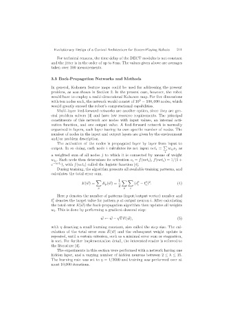
During training, the algorithm presents all available training patterns, and
calculates the total error sum.

1 p p 2
E( w)= E p ( w)= (o − t ) . (4)
i
i
2
p p i
Here p denotes the number of patterns (input/output vector) number and
p
t denotes the target value for pattern p at output neuron i. After calculating
i
the total error E( w) the back-propagation algorithm then updates all weights
w i . This is done by performing a gradient-descend step:
w ← w − η∇E( w), (5)
with η denoting a small learning constant, also called the step size. The cal-
culation of the total error sum E( w) and the subsequent weight update is
repeated, until a certain criterion, such as a minimal error sum or stagnation,
is met. For further implementation detail, the interested reader is referred to
the literature [4].
The experiments in this section were performed with a network having one
hidden layer, and a varying number of hidden neurons between 2 ≤ h ≤ 15.
The learning rate was set to η =1/2000 and training was performed over at
most 10,000 iterations.