Page 213 - Innovations in Intelligent Machines

206 S. Pr¨uter et al.
Stages one and two were repeated for twelve different values of ϕ.The
corresponding correction values for wheel 1 and drift values ∆ϕ are plotted
in Fig. 5 and Fig. 6, respectively.

2.3 Self-Organizing Kohonen Feature Maps and Methods

Since similar friction and slip values have similar effects with respect to the
moving path, self-organizing Kohonen feature maps [3, 4, 6] are the method of
choice for the problem at hand. To train a Kohonen map, the input vectors x k
are presented to the network. All nodes calculate the Euclidean distance d i =
x k − w i of their own weight vector w i to the input vector x k . The winner,
that is, the node i with the smallest distance d i , and its neighbors j update
their vectors w i and w j , respectively, according to the following formula
w j = w j + η ( x j − w j ) · h (i, j) . (2)

Here h(i, j) denotes a neighborhood function and η denotes a small learn-
ing constant. Both the presentation of the input vectors and the updating of
the weight vectors continue until the updates are reduced to a small margin.
It is important to note that during the learning process, the learning rate η
as well as the distance function h(i, j) has to be decreased. After the training
is completed, a Kohonen network maps previously unseen input data onto
appropriate output values.
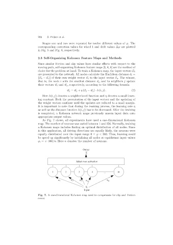
As Fig. 7 shows, all experiments have used a one-dimensional Kohonen
map. The number of neurons was varied between 1 and 256. Normally, training
a Kohonen maps includes finding an optimal distribution of all nodes. Since
in this application, all driving directions are equally likely, the neurons were
equally distributed over the input range 0 ≤ ϕ< 360. Thus, learning could
be speed up significantly by initializing all nodes at equidistant input values
ϕ i ← i · 360/n. Here n denotes the number of neurons.

Output
Y i

Select max activation

1 2 3 4 ... m

w 1 w 2 w 3 w 4 w m

X i
Input
Fig. 7. A one-dimensional Kohonen map used to compensate for slip and friction
errors