Page 260 - Solutions Manual to accompany Electric Machinery Fundamentals

disp (['Ea = ' num2str(Ea(ii)) ' V']);
disp (['Vt = ' num2str(Vt(ii)) ' V']);
disp (['If = ' num2str(i_f(ii)) ' A']);

% Plot the curves
figure(1);
plot(i_f,Ea,'b-','LineWidth',2.0);
hold on;
plot(i_f,Vt,'k--','LineWidth',2.0);
% Plot intersections
plot([i_f(ii) i_f(ii)], [0 Ea(ii)], 'k-');
plot([0 i_f(ii)], [Vt(ii) Vt(ii)],'k-');
plot([0 i_f(ii)], [Ea(ii) Ea(ii)],'k-');
xlabel('\bf\itI_{F} \rm\bf(A)');
ylabel('\bf\itE_{A} \rm\bf or \itV_{T}');
title ('\bfPlot of \itE_{A} \rm\bf and \itV_{T} \rm\bf vs field
current');
axis ([0 5 0 150]);
set(gca,'YTick',[0 10 20 30 40 50 60 70 80 90 100 110 120 130 140
150]')
set(gca,'XTick',[0 0.5 1.0 1.5 2.0 2.5 3.0 3.5 4.0 4.5 5.0]')
legend ('Ea line','Vt line',4);
hold off;
grid on;

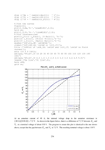
At an armature current of 40 A, the internal voltage drop in the armature resistance is


 40 A 0.18  7.2 V . As shown in the figure below, there is a difference of 7.2 V between E A and
V T at a terminal voltage of about 110 V. The program to create this plot is identical to the one shown
above, except that the gap between E A and V T is 7.2 V. The resulting terminal voltage is about 110 V.

254